Last Updated on 7 January 2026

Portfolio Management takes you through the journey of transforming uncertainty and risk into strategic investment decisions, tracing the field’s evolution from early 20th‑century theories to modern applications.

It defines core concepts, explores public securities markets as information engines, and dissects influential frameworks- from Modern Portfolio Theory and the Fama‑French Five‑Factor Model to Behavioral Portfolio Theory and risk‑parity approaches, highlighting how each model informs real‑world portfolio construction.

This text also delves into the psychological biases that shape investor behavior and offers a hands‑on guide to constructing, measuring and optimizing portfolios, covering return and risk metrics as well as strategy design.

By weaving together theory, behavioral insights, and practical examples, this text equips investors with a toolkit for making better investment decisions.

Foreword

The management of investment portfolios has long been central to achieving financial success, balancing risk, and optimizing returns. Over the decades, portfolio management has evolved from basic asset allocation strategies into a sophisticated field driven by mathematical models, behavioral insights, and, more recently, machine learning and automation. As markets become increasingly complex, driven by globalization and technological innovation, understanding the core theories behind portfolio management has never been more critical.

This paper delves into the most influential portfolio management theories, from Modern Portfolio Theory (MPT) to contemporary frameworks like the Fama-French Five-Factor Model and Behavioral Portfolio Theory. These theories provide the foundation for understanding how investors can optimize their portfolios by managing risk, leveraging diversification, and anticipating market behavior. While traditional models emphasize rational decision-making and risk-return optimization, modern approaches increasingly incorporate behavioral finance and the limitations of human rationality, reflecting the realities of today’s dynamic financial environment.

In an age of algorithmic trading, robo-advisors, and the rise of decentralized finance (DeFi), the practical application of these portfolio management theories is constantly evolving. Investors and portfolio managers must navigate a world where artificial intelligence and machine learning are being used to automate decision-making, while also accounting for human biases and unpredictable market shifts. As such, the need to understand the strengths and limitations of these theories has become more important than ever before.

Throughout this paper, we will not only explore the theoretical underpinnings of portfolio management but also examine how these frameworks are applied in practice. By understanding the history, methodology, and real-world implications of these models, investors can make more informed decisions that reflect both the potential for reward and the inherent risks of modern financial markets.

Introduction

Portfolio management is a deep and fascinating discipline that deals with uncertainty, risk, return and financial decision making, with underlying theories going back to the early 1900s.

In this text we start by defining some key portfolio management concepts, briefly discuss stock markets and then dive deep into some prominent theories that lay the foundations for managing portfolios. We will then discuss psychological biases and wrap up with a discussion of the Portfolio. In this text I mainly discuss securities, which are financial instruments that hold value, and for this reason will sometimes refer to them as “assets” as well. Securities can refer to both publicly-traded and privately-held assets, and in this text I focus on the publicly-traded part.

Basically, the public security markets are a large and sophisticated system of converting information to value and price. It is the mechanism that provides the economy with (noisy) information about its current preferences and needs, and the current state of meeting them. It also provides information about the market’s prediction of the economy’s future needs. Along with creating valuable information, the markets are the best system for distributing resources in the economy, creating physical, true economic growth.

As I briefly mentioned above, investors are rewarded for the correct “reading” of the economy in the form of return. Each investor reads his environment, tries to identify unmet needs and acts to create a position, and while they are doing so they act as a single brain, constantly receiving information and trying to understand where resources should be allocated. If an investor is correct, they receive a return that is connected with the benefit they created for the economy. While some investors win and others lose, the system itself benefits from this concerted effort of transforming information into resource allocation decisions.

Return is strongly connected with the risk investors take. Quality information is not easily available among all the noise and the ability to process it is precious. It’s very difficult to really understand the system around us and the return is its way of incentivising its thinking members. As we will see in this text, risk and uncertainty come from lack of information, and the need to still make decisions in such environment. So, as investors take risks and deal with uncertainty, the system rewards them for correct decisions.

Since this reward is connected with risk, if there was more quality information and better ways to process it and really understand the coming capital needs of our economy, there was less risk, the markets would be more efficient and the overall return would be lower.

Let’s briefly discuss the most basic topics in portfolio management:

What is “investing”?
Investing is the act of putting capital to use today through getting exposure to assets, with the expectation of a future return. Investing is basically the distribution of value across the system for constructive purposes, with the aim of creating more value in the future. It can be executed through taking a debt or equity exposure to an asset, or through a derivative.

What is “return”?
This is the reward the system grants investors for sustaining and improving it while taking risks. We earn a return when we make solid investment decisions. It manifests either as our asset’s valuation grows (capital return), or when it distributes cash (yield) among any other potential benefits. Therefore, a return can be thought of as all the benefit we get when we own an asset. Return is always time-dependent and measured between two point in time.

What is the goal of portfolio management?
The goal is to maximize return on invested capital for a given level of risk tolerance, or to minimize risk for a given level of desired return. This is done through analysis of information, decision making and the subsequent creation of a portfolio, which represents the investor’s total investment exposure positioning that consists of one or more securities.

Who manages portfolios?
Portfolios can be managed by the investor himself, by a human professional or a robo-advisor, which is an automatic portfolio management service. No matter who manages a portfolio, the same principles apply: everyone tries to figure out the best investment opportunities in their views and to create a position that gains if their predictions come true, while trying to minimize losses if their predictions turn out to be false. All while having the investor’s goals and constraints in mind.

Who invests in publicly-traded securities?
3 main groups of investors:

• Institutional Investors- these are basically large entities that manage other people’s money mainly for the long-term. The core of this group includes pension funds, insurance companies, foundations, endowments and sovereign wealth funds. What mostly characterizes institutional investors is their patience. For this reason, institutional investors are perfectly positioned for investing in Alternative Investments.
  
• Significant Players- these are other institutions that are influential in the markets but are not necessarily patient or take a long-term view to investing. This group includes banks and other savings management entities, mutual funds, hedge funds and also municipal and national government agencies.
  
• Retail investors- these are non-professional individuals who invest their personal savings in publicly traded securities. They invest smaller amounts and while acting alone, as a group they constitute an influential part of the asset markets. In recent years, this group was responsible for 20% to 40% of overall trading volume^◆.
  
  The following chart shows the share of total trading volume in the 2010s by the aforementioned investor groups:
  
  
  ^{Source: The Economist- Just how mighty are active retail traders?}
  
  The COVID-19 trading spike by retail investors is clearly visible for the 2020-2021 figures. It’s important to note that it seems like different sources count different investors under the definition of “retail”. No new information about 2022 and 2023 is yet to be published.

With capital markets being a machine for the analysis-based distribution in the economy, the market gets what it wants in the short-term, but what it needs in the long-term.

Definitions

Before diving into portfolio management, I wish to define some basic terms that will support the discussion. This section is divided into three parts:

1. Portfolio Management Definitions- as its name suggests, this part defines terms relating to the management of security portfolios.
2. Capital Markets Definitions- this part defines terms relating to capital markets in general.
3. Statistical Analysis Definitions- statistical analysis provides a set of tools to analyze data. Portfolio management relies on the past to make predictions about the future, and statistical analysis allows us to do so methodically.

Portfolio Management Definitions

Security (plural: Securities)- this basic term describes financial contracts that hold monetary value. Each security is a contract, since it grants its owner some rights and obligations in an economic asset.

There are four types of securities:

• Equity- these contracts provide ownership rights to their holders, such as common stock or partnership units.
• Debt (“fixed income”)- these contracts provide their owners the right to receive periodic principal + interest payments from the debtor, such as government, municipal or corporate bonds.
• Hybrid- these contracts involve both equity and debt aspect, such as convertible bonds, warrants and preferred shares.
• Derivatives- these contracts provide many kinds of rights to their holders. They can be versatile and specific. But basically, these contracts’ value is derived from the value of an underlying asset. For example: futures, options, swaps and forwards.

Securities can be viewed as a specific type of assets, in that they are financial assets. They can be publicly-traded or privately-held.

In 1946, the U.S. Supreme court established the “Howey Test”, which was used to determine whether an asset constitutes an investment contract (a security). The test consists of four criteria: an investment of money, expectation of profits, common enterprise and reliance on the efforts of others. This test is used to this day: if an asset qualifies all 4 criteria, it is considered a “security” and falls inside the scope of the U.S. Securities laws.

An Efficient Portfolio- this is a portfolio that provides the greatest expected return for a given level of risk, or the lowest risk for a given expected return (Theory and Practice of Investment Management, Second Edition, p. 6)^◆. To construct an efficient portfolio, we need to be able to quantify and predict future risk and understand the expected return of various securities, and how their behaviors interact.

A Portfolio- this is a collection of securities an investor owns. Security ownership is stored in an electronic form within a central depository, such as the Depository Trust & Clearing Corporation (DTCC) in the United States, the Canadian Depository for Securities (CDS) in Canada, and the Tel Aviv Stock Exchange Clearing House in Israel.

A Position- this term describes an investor’s current financial exposure to new information generated in the financial markets. A position is created by buying assets, as each asset is sensitive to different information and reacts differently to event that occur in the environment. The position is the investor’s total exposure to such information, as derived by his portfolio assets’ aggregate exposures.

Investing- this is the popular name for the action of “putting capital to use today with the expectation of receiving a return in the future”. When we invest, we expose ourselves to both value creation and investment risks and if all goes well, we receive a reward in the form of return. Investing is always made as ownership rights in securities that offer exposure to various assets and entities. The goal is always to generate a return on capital. The only true source of return is a successful creation of value, both through the underlying asset and in its environment. See an elaborate discussion of what is an asset in my text Asset Valuation.

Investment Risk- as per Frank Knight’s definition of uncertainty and risk (this is discussed later under “Risk, Uncertainty and Profit“), Investment Risk refers to the possibility that while we may be able to project probabilities of different outcomes for our portfolio, based on past data, there is a chance we will not achieve the goals we set to ourselves when creating it.

Investment risk sits at the base of the employment of capital. It is for the uncertainty and risk that we get offered a return. Extensive empirical evidence suggests a direct connection between the two.

Risk Premium- this is the extra return above the risk-free rate investors require in order to agree to expose themself to the risk of holding a riskier investment. This concept helps explain why equities typically have a higher return over bonds and why alternative investments often offer returns that are even higher, due to the illiquidity premium, a type of risk premium.

Leverage- this term refers to the use of borrowed capital in order to increase investment exposures, aiming to increase the investment base and amplify the potential returns on investment, as measured against the investor’s initial capital. This tool can significantly enhance the potential for higher returns but also comes with higher risks.

Leverage basically involves obtaining a loan in order to increase our investment exposures. It works like this: the investor brings his own capital, referred to as “equity”, into the investment, and can borrow more capital which will allow him to get a greater exposure to various assets. If the investment succeeded, they will repay the loan and keep the rest. If it failed, they will lose some or all of their equity and still need to return the borrowed principal + interest + fees. Like always, the investor would like the loan to be as cheap as possible. Leverage can also come in the form of broker margin loans or financial derivatives. It’s any situation when the investor may end up owing money in a future point in time and uses this money today to invest. It looks like this (gross returns and no interest rates on debt):

This example shows a hypothetical scenario of using 75% leverage to get exposure to a security. The left chart shows what happens when the security gains 50% Return on Investment (ROI), which the same as the Return on Assets (ROA). In this scenario, the return on the investor’s equity (ROE) is much greater, 200%, before considering debt costs. The right chart shows what happens when the security losses 50% ROI (ROA). Our equity loss is triple that amount, -200%, wiping the investor’s initial capital and leaving him owing the remaining debt + interest.

The total investment exposure is equal to the initial capital plus borrowed funds. Therefore, the use of 75% leverage creates a total investment exposure of $4 for every $1 of initial equity capital.

This relationship between ROE and ROA when using leverage can be summarized in the following way:

Where:

is the leverage ratio, the ratio between total initial investment value and the investor’s equity, or .

is the interest rate paid on leverage, as measured on the same time period as the ROE and ROA.

When debt is involved, we refer to our ROE as “levered ROE” to highlight its increased risk exposure.

As we have seen, we employ leverage to alter our portfolio’s exposures to risk. When measured by standard deviation of returns, this change can be approximated by:

When we use leverage to increase our exposure to some or all securities in our portfolio, their weights, relative to our initial equity capital, will grow to be larger than 100%.

Volatility- this measures the rate of fluctuations in the price of a security during a time period. It refers to the degree of variation in periodic security returns over time. In investing, this typically refers to the standard deviation of a security’s returns over a past time period. Higher returns mean a higher volatility.

Volatility Drag- this term refers to the negative effect that fluctuations in returns have on an investment’s long-term growth. When an asset experiences volatility, losses require proportionally larger gains to recover, which makes it harder for the investment to bounce back fully. This results in the compounded return, or the actual return over time, being lower than the arithmetic average of periodic returns. Volatility drag can significantly reduce an investment’s final value, as the real growth is hampered by the compounding effect of both gains and losses.

For example, if you invest $100 and lose 50% in the first year, your investment drops to $50. Even if you gain 50% in the second year, your investment only rises to $75, not back to $100. The arithmetic average return suggests 0%, but the actual compounded return is negative due to volatility drag. This illustrates that the compounded return (IRR) is the more accurate measure of performance, as it reflects the real impact of volatility and losses on your investment’s value over time.

Asset Class- this is a group of investable assets that share similar characteristics, behaviors and risk exposures. Investing in a healthy amount of asset classes is considered to be good practice for diversification and a balanced exposure to systematic risks. For example: equities, fixed income, real-estate, currencies, commodities or the various classes of Alternative Investments.

Asset Allocation- this is the action of distributing given capital between various strategies or asset classes based on the investor’s expected return and risk preferences. The result is a diversified portfolio of assets that represent exposures to different risks.

Alternative Investments- as I thoroughly explain in my text about Alternative Investments, these assets can basically be defined as all the economic objects and entities that are not publicly traded in a stock market. Most of the times, these assets are harder to trade and are therefore considered “illiquid”, offering illiquidity premium to investors which suits great with patient institutional investors. In order to get exposure to such assets, investors usually need to act differently and work with intermediaries in order to find and manage investments. Examples of alternative investments are various assets of private equity, private debt, infrastructure, real-estate and more.

Liquidity– this term describes how fast one can transform his asset into cash without a major influence on the price. Low liquidity means that in order to buy or sell an asset, the investor needs to work harder and compromise on the price, often paying higher transaction costs. Publicly-traded securities usually have more liquidity and are easily traded than privately-held assets, that often need special intermediaries for execution.

Illiquidity Premium- this is the extra return investors require to get in order to agree to lock their capital for longer terms, with little ability to trade their asset, such as the case with privately-held assets (contrary to publicly-traded assets). This means that investors expect to receive higher returns from illiquid alternative investments, or else they would not make a deal.

Endowment- this is a type of institutional investor. It is a pooled capital management entity, meaning it has a team that collects and manages capital on behalf of other people. An endowment’s aim is to use its capital to benefit a specific individual or organization, often of educational or charitable nature, with capital preservation in mind. Basically, it invests capital it receives from various sources, such as donations or other revenue sources, and distributes the returns to the individual or organization for its various needs. Oftentimes, endowments are tied to an institution’s spending policy, which aims to spend a certain part of the endowment per year while maintaining or growing capital. The endowment’s management tries to earn enough real returns to cover annual withdrawals and preserve the real value of their principals.

Arbitrage- in its purest form, is defined as an opportunity to gain profit without taking any risk. This means that the profit is guaranteed and there is zero risk of a loss. This concept is implemented in the real world by exploiting information inefficiencies as quick as possible and often includes some kind of little risk. Speed is paramount as we need to act faster than the rest in identifying the opportunity, processing the information, making a decision and creating a position. In reality, pure arbitrage is very rare and some risk always exists in any trade.

Arbitrage offers the financial system many benefits: price alignment across markets, increased market efficiency, liquidity provision, reduced price volatility, improved integration of different markets and a beneficial feedback mechanism- where in their actions, arbitrageurs provide information about market inefficiencies.

The Risk-Free Rate of Return- in theory, this is the return of an investment with zero risk. In practice, this is the periodic return on the safest asset in the economy which is usually government bonds. This return is usually stated in annual terms and taken from the relevant future period in the Term Structure of Interest Rates, that states the yield to maturity on a specific type of government bond. Like most return figures, it is measured on an annual basis.

Market Capitalization- this is the total market value of a publicly-traded entity’s equity. It is basically the result of multiplying the entity’s outstanding shares with its share price. This is the entity’s equity value, and adding the total outstanding debt to this figure will generate its enterprise value.

Alpha (α)- this term describes investment outperformance, the return we achieve beyond what we expect to receive. It is measured by any excess return generated above a benchmark index or above a return projected by a model. In other words, it represents our ability to generate returns above what would be expected given a model or compared with a benchmark. Alpha basically refers to the part of a portfolio’s return that is not a result of the general market movement.

In literature, alpha, in the context of systematic risk exposure, is explained as excess return achieved due to incomplete models. In the context of information alpha through idiosyncratic risk exposure, alpha is achieved through superior information collection and analysis in non-perfectly efficient markets. The emphasis is on the investor’s true unique capabilities, as they are tested in multiple periods, where luck is expected to equal zero.

Like with any analysis of investment returns, in order to make alpha more complete, we must introduce risk. Returns must always be considered in the context of the risk taken, so discussing alpha without accounting for risk is misleading. There is another concept of alpha that takes risk into account as well- Jensen’s Alpha, which I discuss under Single-Index Performance Measures hereunder.

Beta (β)- this term refers to a security’s sensitivity to a factor, which is some state in the world that affects security return behavior. It is calculated as the slope of the least-squares line (the regression line) of a plot depicting the periodic return of securities that represent the factor (x, explanatory variable) and a portfolio’s periodic return (y, dependent variable). I will discuss this term more deeply under Factor Models hereunder.

Benchmark- in portfolio management, this is a reference point against which the performance of a portfolio can be compared. These are usually indexes that represent markets or industries, and we use them to compare our portfolio’s expected and actual risk and return. By selecting an appropriate benchmark and comparing its performance with portfolio, we could know if did a good job in our investing, such as whether we were able to “beat the market” by achieving a higher return, or even better, by achieving a better return-risk ratio. Common benchmarks: the S&P 500 for the US equity market and the Bloomberg Barclays U.S. Aggregate Bond Index for the US bond market.

Long Exposure- the traditional form of exposure, when we profit from an increase in an asset’s value. It is achieved by buying an asset. Also known as “long position”. For example: equity, bonds and “call” options.

Short Exposure- when we profit from a decrease in an asset’s value. Also known as “short position”. It is achieved by “selling short” an asset, meaning borrowing it, selling it and committing to buy it again at the market rate in future time, profiting from any decrease in price. a For example: short selling, put options and insurance policies.

Technical Analysis- this is a method to study and predict future security price movements using past trading data. This method tries to identify trends or patterns that could perhaps tell us something about the security’s future price movement. It focuses on past price charts, various ratios and some more complex calculations to try and predict the next period’s price movement.

Fundamental Analysis- this is researching an asset’s “fundamentals”, its KPIs, through using information from financial statements and other public sources. This is a qualitative analysis that tries to have a deeper understanding of an asset, make a valuation and support an investment decision.

Active Investment– this is a “hands-on” approach to portfolio management. Active strategies depend on the portfolio manager’s ability to collect and digest vast amounts of information and be able to tell which securities and industries will outperform the others. They include the buying and selling of securities with the aim of outperforming the benchmark market. The goal of these strategies is alpha (α), excess return over the market through skill.

Passive Investment– strategies rely on diversification to match the performance of some market index. They are basically implemented by the buying and holding of Exchange Traded Funds (ETFs), which are an affordable and efficient way to gain diversification. These strategies are based on the assumption that “the market knows best”- prices include all available information and there is no use in trying to beat the market. The goal of these strategies is beta (β), the market risk. Passive investing prevents investors from benefiting from skill in recognizing inefficient security pricing.

Trading Volume- this is the total number of security units, such as shares, that switched hands in deals during a period.

Trading Turnover- this is the total cash that switched hands in deals during a period. It is calculated by summing the multiplication of each deal’s number of units and their price.

Dynamic Correlations- securities show correlations in their return behavior over time, as some securities are more related and are exposed to similar risk factors. For example, securities that belong to the same sector are projected to act relatively similar in face of new information from the environment. However, the nature of these relationships naturally changes over time, as the companies and markets evolve. It can even happen abruptly in times of market stress, when most securities start showing a strong positive correlation and drop together. Recognizing that correlations are dynamic is important for a more true view of a portfolio’s positioning and for more efficient risk management.

Bid-ask Spread- this is the difference between the highest price that a buyer is willing to pay for a security and the lowest price that a seller is willing to accept. The bid price is the maximum price a buyer is willing to pay for a security. The ask price is the minimum price that a seller is willing to accept to sell a security. A lower spread means a more efficient market and a more liquid security. Some securities show a lower spread, most show a higher spread.

An Option- this is basically a contract that grants its owner the right, not the obligation, to do something. This right is worth money and therefore options have a price. Holding a financial option grants it owner an exposure to the price of an underlying asset. This exposure can be long, as in a call option, or short, as in a put option. The investor’s profit comes from the difference between the underlying asset’s price stated in the option contract and its current market value. Options always have an expiration date, which indicates the last or only date the option can be exercised. The Owner always have the option to not exercise the option.

Call Option- grants its owner the right to buy the underlying asset at a predetermined price, no matter what its current market price is.

Put Option- grants its owner the right to sell the underlying asset at a predetermined price, and again no matter what its current market price is.

Ex Post- this is a Latin term that means “after the event”. In finance and investing, it is used to describe backward-looking analyses, evaluations or performance measurements after they have occurred. Basically, this term relates to explaining and learning from the past in order to increase our wisdom.

Ex Ante- this is a Latin term that means “before the event”. In finance and investing, it is used to describe forward-looking analyses, predictions and forecasts that are made before the occurrence of a specific event or before certain data becomes available. Basically, this term relates to making predictions.

It is important to distinguish between the two terms when managing portfolios. Oftentimes, people mix past analysis with future outcomes, such as the case when they discuss a security’s standard deviation of returns: this figure is derived ex-post and its use implies the assumption that it will remain the same ex ante, in the future. This is an assumption that often doesn’t hold. We convert uncertainty to risk when we learn from the past and use what we learned to predict the future.

In portfolio management, we often use past data in order to better understand a position and make forward-looking predictions. In time-series analysis, where we collect price observations in set time intervals, we face with the choice of our dataset’s past data time-granularity. This means we need to decide whether to take an observation every minute, day, week, month, etc. We can possible choose to take another strategy and take a measurement every certain trading volume.

The decision on past data granularity depends on and directly proportional to our future prediction timeframe: i.e. if we seek to maintain positions for a very short time, we should analyze data at very short time intervals, and the opposite for long holding periods. Highly-granular data comes with higher noise, but the more specific the predictions can become, as it provides a more detailed insight into patterns and anomalies. We seek to balance specificity with noise and match our past data granularity with our expected holding period. Most of the time it is possible to convert high-granularity data to lower-granularity data, while the opposite is not possible.

Capital Markets Definitions

Capital markets is a general name for the industry of resource allocation, where investors of all types trade securities. The following definitions explain some key terms in this field:

Publicly-Traded Securities- these are all securities that are traded by the public in an exchange. Publicly-traded assets are subject to strict regulatory requirements, including regular financial reporting and disclosures.

Privately-Held Securities- these are all securities that are held private, meaning they are not publicly-traded. Oftentimes, regulation on privately-held securities is more lax and information is more scarce.

Primary Market- this is when entities issue securities and sell them to the public, with the goal of raising capital to fund their operations.

Secondary Market- this is when existing securities change ownership. These securities were already created in the past by an an entity and are now traded between an existing owner and someone else. The issuing entity does not get any direct gain from a secondary market deal, but the system gets information on how market participants perceive the entity’s value, as such a deal results in a security price that can be translated to valuation.

The Law of One Price- this theory refers to the idea that the price of a security or asset will have the same price no matter where it is traded, based on several assumptions, such as efficient markets, perfect information distribution and free and frictionless trade. According to this theory, in the most efficient markets, arbitrage opportunities should eventually lead to the convergence of prices in different markets, as arbitrageurs buy the security where it is cheap and sell it where it is expensive. In reality there are many frictions and distortions in markets that keep a gap between the prices of the same securities traded in different markets.

Exchange Traded Fund (ETF)- this is a type of publicly-traded security that holds claim to an underlying pool of assets. It provides investors the ability to get exposure to groups of assets through buying a single security. For their service, ETFs charge fees. For examples, ETFs can provide exposure to a market index like the S&P 500, to commodities like gold and oil, and even Bitcoin and Ethereum. Some ETFs offer an inverse relationship with the underlying asset pool by using short selling and derivatives.

A Bull Market- this term refers to an optimistic perception of markets, whereby participants expect economic growth, investor confidence, higher trading volumes and rising security prices for a period between several months to a few years. Bull markets are caused by a benign economic environment such as declining interest rates, strong economic indicators and better government policies.

A Bear Market- this term refers to a pessimistic perception of markets, whereby participant expect economic decline, investor inconfidence, lower trading volumes and falling security prices for a period between a few weeks to several years. Bear markets are caused by an adverse economic environment such as rising interest rates, inflation, weak economic indicators, geopolitical crises or worse government policies. A bear market is often defined as a drop of 20% or more from recent highs.

Yield to Maturity (YTM)- fixed income instrument prices are influenced by market supply and demand and since their coupon is fixed, their yield to maturity changes with their price through an inverse relationship. A bond’s yield to maturity is the annual yield it will generate until it matures, based on its remaining coupons, its face value and its purchase price. When the bond matures, the issuer pays the face value to the bondholder.

The YTM is similar to the bond’s internal rate of return, its IRR. It’s important to note that like IRR, YTM assumes all future coupon payments are reinvested at the same rate as the current yield.

Term Structure of Interest Rates- also called the “yield curve”, this is a representation of the different yields to maturity of debt securities, usually government bonds, with different maturities. The information is shown either in a table or a chart, where the x-axis represents time to maturity and the y-axis represents the yield to maturity.

Since this concept represents the yield to maturity of publicly-traded debt instruments, it incorporates investors’ current expectations about the future as they manifest in current bond prices.

Internal Rate of Return (IRR)- is an estimate of an investment’s annual rate of return that takes the time value of money into account. It is the specific discount rate that makes an asset’s Net Present Value (NPV) equal to 0, meaning it’s the rate at which the present value of future cash flows equals the initial investment. The IRR can be interpreted as an annualized return on invested capital, since it essentially tells us what annual return we would need to get in order to break-even on our investment. It looks like this:

Where:

is our initial investment.

is the net periodic cash flow.

is the discount rate that solves this equation.

Notice that our initial investment is given as the cost to create our portfolio and the cash flows are given as time passes and yield is distributed to the portfolio owner. The last cash flow is the portfolio value at the time of measurement, as we pretend to dissolve it and distribute the proceeds for the calculation. The only thing that adjusts and depends on those figures is the IRR. This is the discount rate and therefore the annual return on investment under any cash flow scenario.

The IRR is useful since it allows us to compare returns from different investments made over a similar time frame, even if the investments are made for different lengths of time or have different cash flow intervals. The IRR calculation includes the assumption that cash flows can be reinvested at the IRR itself. It is a volatile figure that depends on the amount and timing of the asset’s cash flows, among other assumptions.

While IRR is useful for cash-flow-driven investments, where cash periodically flows in and out of the portfolio, it can’t be directly compared with the Time-Weighted Return (TWR) used for publicly traded assets. IRR is investor-specific, capturing the impact of individual cash flows and timing, while TWR is asset-specific, measuring the return an asset generates over consistent time intervals. TWR isolates the asset’s performance independently of external cash movements, providing a standardized return measure for liquid assets. By contrast, IRR’s cash flow sensitivity, tailored to individual scenarios, can distort comparisons with publicly traded asset returns.

Statistical Analysis Definitions

Statistics plays a crucial role in managing portfolios, since it provides the mathematical foundation necessary to analyze and interpret financial data, assess risks and make investment decisions that are based on past experience. The following definitions explain some key terms in this field:

Variance- this is a statistical measure that is calculated on past periodic data and measures the dispersion of data points around their mean. In investing, it is used as a proxy for risk, since the higher the variance of security returns, the greater the uncertainty and thus the higher the risk associated with the investment. In practice, we use the standard deviation of returns, which is the square root of variance, because it is depicted in the same unit as the underlying sample units- periodic returns.

Variance, when measured on a sample of observations, is calculated as follows:

Where:

is the standard deviation of our observations’ data points. is the variance.

is a data point.

is the sample mean.

is the total number of observations.

Covariance- this is a statistical measure that is calculated on past periodic data and indicates the extent to which two variables change together. It is positive when the two variables tend to move together, and negative if they tend to move on opposite directions. Like variance, covariance is not limited to a specific range. With regards to security returns, it is calculated using any of the following identical methods:

Where:

is the correlation of past periodic returns of securities and .

are the periodic return of securities and in period .

are the average periodic return of each asset as calculated in our lookback timeframe.

is the number of periods in our sample.

We basically calculate the difference between the return of asset in period and its mean return over the lookback period, the difference between the return of asset in period and its mean return over the lookback period, sum these differences and normalize by dividing with (and not ). This adjustment is called Bessel’s Correction. It’s made to account for the fact that we are calculating the volatility and average on the same sample, reducing the number of independent pieces of information by one.

When we calculate the covariances of pairs of securities, we can put the results in a table and call it the covariance matrix, where each row and column represents a security and the intersection between two securities shows their covariance. The diagonal line from top-left to bottom-right in this matrix shows each security’s variance.

Annualization- in finance, annualized values are the standardized way of measuring investment characteristics. They provide a consistent basis for interpretation and make it easier to compare with other annualized figures, as comparing values is only meaningful when they describe behavior over the same time span. Annualization gives us a more realistic picture of an asset’s performance over time.

When analyzing an asset’s past returns without compounding (i.e., no exponential growth due to reinvestment of returns), we often annualize by multiplying the observed return by the amount of periods within a year: 252 for daily data, 12 for monthly data.

When compounding is involved, simply multiplying returns by the number of periods would overlook the effect of reinvestments. In such cases, we annualize by calculating the geometric average of the periodic returns, which does account for the compounding effect over time. See Annualizing Returns hereunder for more information.

For volatility, we will always annualize by multiplying the variance by the same number of periods. However, for standard deviation, we take the square root of that number instead, as volatility scales differently.

We will annualize our asset’s performance values when we need to compare between different assets on the same basis and when modelling our portfolio’s performance, just for consistency and clarity. Regulation often also requires annualized figures.

We can avoid annualization of our asset’s performance figures if we focus solely on the short-term, such as a week or shorter.

Correlation- this is a statistical measure that is calculated on past periodic data and measures the extent to which to variables are linearly related. It quantifies both the strength and the direction of the relationship between two variables. Correlation has 3 main types:

1. Pearson Correlation- this is basically a normalized covariance, making it independent of the scale of the variables, allowing for a standardized measure of the strength and direction of a linear relationship. It is capped between -1 and 1 and assumes both variables are normally distributed and that the relationship between them is linear. It is sensitive to outliers. This coefficient is used when the relationship between the variables is linear and the variables are roughly normally distributed.
   
2. Spearman’s Rank Correlation- this correlation coefficient is a non-parametric measure that assesses how well the relationship between two variables can be described using a monotonic function. It is based on the ranks of the data rather than their raw values. It is not tied to linearity, making it suitable for ordinal data or non-linear relationships. It does not require the data to be normally distributed, so it fits these instances as well. It is also capped between -1 and 1. It is less sensitive to outliers than the Pearson correlation.
   
3. Kendall’s Tau- this correlation coefficient is a non-parametric (it may be more versatile but less powerful) measure that assesses the strength and direction of association between two variables. It is calculated based on the number of concordant and discordant pairs among all possible pairs in the dataset. It’s suitable for ordinal data, variables that do not have a linear relationship and for data that is not normally distributed. It is also capped between -1 and 1.

For these correlation coefficients, a score of 1 is considered to indicate a perfect positive relationship, -1 a perfect negative relationship and 0 no relationship.

Linear Relationship- this refers to the situation when a change in one variable is associated with a proportional change in the other variable, either in the same or opposite direction. This relationship can be represented graphically as a straight line on a scatter plot, where one variable is plotted on the x-axis and the other on the y-axis.

Monotonic Relationship- this refers to the situation when two variables move in the same single direction but not necessarily at a constant rate. This means that as one variable increases, the other either consistently increases (positive monotonic relationship) or consistently decreases (negative monotonic relationship). Such relationship is “monotone” but not necessarily linear: a change in one variable can be related to a change in the other variable that gets more or less intense over time.

Ordinal Data- this refers to categorized data organized by ranking, but the intervals between the categories are not necessarily equal or known.

Regression- referred to as “regression analysis”, this is a statistical method used in data analysis to model the relationship between a dependent variable, often denoted as , and one or more independent variables, often denoted as . The goal of the regression is to predict the value of the dependent variable based on the values of the independent variables. The result of the analysis is basically a mathematical equation that describes the value of based on the values of the s and a corresponding coefficient, typically denoted as , that represents the weight of each in explaining .

Regression is widely used in portfolio management to model relationships between independent and dependent variables.

A linear regression looks like this:

Where:

is the dependent variable, the value we are seeking to predict.

is the regression’s intercept, the dependent variable’s value when all the independent variables’ values are 0.

is the sensitivity coefficient of independent variable .

is the error term, accounting for the difference between the observed and predicted values of Y.

Contrary to the liner regression model, non-linear regression assumes non-linear relationships between the independent variables and the dependent variable in the data. Such relationships can manifest as polynomial, exponential, logarithmic, trigonometric, power law among other relationships. The goal is to explain the underlying data with a mathematical formula with as little error as possible to catch its characteristics, while avoiding overfitting to maintain generalized predictive power.

The following graphs show an example linear and an non-linear regression lines with a high explanatory power:

R-Squared ()- also known as the coefficient of determination, this is a statistical measure that quantifies the proportion of the variance of a dependent variable that is predictable from one or more independent variables in a regression model. Basically, it provides a quantitative measure of the fit of the model to the actual data. R-squared ranges from 0 to 1, with values closer to 1 indicating a strong model fit, suggesting that the model explains a large proportion of the variance in the dependent variable. In the context of a simple linear regression, R-Squared is the square of the Pearson correlation coefficient between the observed values of the dependent and independent variables.

It looks like this:

Where:

the residual sum of squares, this is the sum of the residuals squared. A residual is each data point’s distance from the predicted point- on the regression line.

the total sum of squares, this is the squared sum of the distance the data is away from the mean. It measures the total variability of the dependent variable relative to its mean, which includes both the variability explained by the independent variables and any unexplained variability.

is the value of a dependent variable, our portfolio’s return in a certain period.

is a regression model’s prediction of our portfolio’s return in a certain period. is our model’s error.

is the average value of the dependent variable in the dataset, our portfolio’s average periodic return. is the difference between each value of the dependent variable and the average value.

It’s important to note that the R-Squared does not indicate the correctness of the regression model and does not disclose information about any causation relationship between the variables. Therefore, this statistic should always be used with other measures of statistical analysis.

Cross-Section Analysis- this term refers to the analysis of data at a specific point in time across different subjects, such as the publicly-traded stocks of a group of entities. It is basically a snapshot analysis of multiple subjects over the same timeframe, in order to identify patterns as we compare between the subjects. This comes in contrast with longitudinal or time-series analysis, that focus on the change in a specific subject over time.

Distribution- this is the way in which values of a variable are spread across a range of possible outcomes. It represents the underlying probability of all possible values a variable can take in a setting. Distributions can be depicted as mathematical formulas, graphs or tables. They describe characteristics such as central tendency, dispersion, skewness and kurtosis of a data sample. There are many types of distributions that describe different phenomena under a set of assumptions, but they are all used to understand the behavior of data and making inferences about a population from a sample of observations.

Histogram- this term specifically relates to the graphic representation of a distribution. It uses bars to show the frequency of data points that fall within each bin. Each time an observation is analyzed, a desired trait is recorded, and we can plot its numerical value in a bar chart. On the chart, the x-axis shows the bins, which are the range of results values divided into identical intervals, and the y-axis shows the number of times each result was achieved. A Histogram is basically the counting of observations and the value of the desired trait in each one. A Histogram is an empirical, practical tool used to visualize the distribution of a dataset.

Normal Distribution (Gaussian Distribution)- this is one of the most important distributions in statistics. It is characterized by a “bell”-shaped curve, symmetry around the mean and that the mean, median and mode are equal. It is therefore fully described by its mean and variance. Like many known distributions used in statistics, it assumes that the traits we measure in a sample taken from a population of observations- are independent. An important use of the normal distribution is made when analyzing the possible movement of security prices during a period, even though periodic returns are not independent of each other. It allows for many important statistical analysis tools and this is the main reason why many theories rest on assumptions that allow the use of this distribution to model the occurrence of the trait.

Skewness- the third moment of a distribution after the mean (first) and variance (second), skewness measures the asymmetry of a distribution around its mean. It primarily assesses how data is spread out. Positive skewness indicates a distribution with an elongated tail on the right side, meaning most observations are concentrated on the left side. The opposite occurs for negative skewness. A positively skewed distribution implies that an investment has a higher potential for outsized gains, even if it also experiences regular losses, and vice versa.

Kurtosis- the fourth moment of a distribution, this measures the “thickness” of a distribution’s tails compared to a normal distribution. This is used to gauge extreme outcomes in the data. High kurtosis indicates a higher probability of extreme positive and negative events.

Z-Score- this statistical measure describes the position of a data point in terms of its distance from the sample mean, measured in standard deviations. In other words, the Z-score standardizes the dataset and quantifies how many standard deviations an individual data point is from its sample’s mean value. Standardization is the process of rescaling the data to have a mean of 0 and a standard deviation of 1, thus converting the data points into units of distance from their mean. Z-score is a way to standardize scores on different scales, so they can be compared directly with other values or used in further statistical calculations. It looks like this:

Where:

is a data point’s value.

is the dataset’s mean value.

is the standard deviation of the dataset around its mean.

The application of Z-score onto a dataset is a kind of standardization, and it enables their analysis based on their distance from their mean, effectively standardizes them into units of distance from the mean. Therefore, Z-score allows for the comparison of scores from different distributions and scales. It is also used to identify dataset outliers, as those will immediately pop up as having high Z-score values. As a rule of thumb, data points that are normally distributed with Z-scores of are considered to be outliers.

In a standard normal distribution, where the mean is 0 and the standard deviation is 1, the Z-score directly corresponds to the data points’ percentile rank, making it useful for parametric VaR calculations. Standardizing any normal distribution converts its values to standardized values that are distributed as a standard normal distribution, allowing us to converge the its Z-score and percentile ranks.

A Z-score of 0 indicates that the value is exactly average, while a Z-score of 1 means the value is one standard deviation around the mean, and so on. A percentile rank of a data point refers to the percentage of data points in the distribution that are equal to or less than that data point.

Vector- generally, a vector is an ordered list of numbers. In mathematics, vectors typically represent a quantity that has both magnitude and direction, which can often be visualized as an arrow pointing from one point to another in space. In statistics, vectors are used to represent data, such as a list representing a trait of various observations in a dataset. In machine learning, vectors represent the values of an explanatory variable (a feature), for different observations. A matrix can be viewed as a list of vectors, connecting them together in an ordered fashion. Matrices and vectors can be added together, multiplied by scalars (which are either real or complex numbers), multiplied by each other (“dot” products), Euclidean Distance and more.

Robustness- this term refers to the ability of a method or model to remain effective under different conditions or assumptions. A robust model is less sensitive to outliers and less dependent on assumptions regarding underlying data distributions. It is expected to perform well not only under ideal conditions, but also under various deviations, such as those arising from real life.

The Stock Market

Stock markets, also called “stock exchanges”, are institutions that facilitate the trading of financial assets. They are basically a regulated mechanisms, where buyers and sellers of securities meet, make offers and accept terms.

As of 2023, there are around 80 major stock markets across the world^◆, up from 60 in 2015^◆. The total market capitalization of the world stock markets rose from USD 2.53 trillion in 1980 to USD 93.69 trillion in 2022, after reaching a record USD 111.16 trillion in 2021^◆. A country usually has at least one stock market, and some of the larger economies have multiple.

Stock exchanges serve as a regulated meeting place for buyers and sellers of securities to meet and trade. There, sellers publish their asking price and buyers publish their bidding price, and if their requirements converge, a deal is formed. The difference between the ask and bid price is called the bid-ask spread.

In the distant past, this meeting was done physically. Later, it was facilitated through intermediaries located in the stock exchange premises, and since 1971 starting with the NASDAQ, trading gradually became fully automatic through electronic means.

The stock markets allow entities to raise capital from investors and employ it to create value. Business entity seek to accumulate human talent, methods and assets. They are experts in creating value in their field of expertise. However, they usually need capital that serves as fuel for their operations and expansion. When these entities are small, they turn to the private capital markets for funding. When they grow, they turn to stock markets by performing Initial Public Offerings (IPOs) of stocks or issue debt. This usually means an exit for the private investors. Well functioning public capital markets are paramount for the economic success of a nation that relies on its people’s hard work.

The government is also an active player in the stock markets, as it uses the platform to sell debt instruments to the public through the issuance of treasury bills, notes and bonds.

The following table shows information about some prominent national stock exchanges:

On top of this list there are also exchanges that focus a single type of financial asset, such as Chicago’s CBOE which was established in 1973 and focuses only on options trading.

Security stock exchanges have been prevalent in Capitalist societies, and have been granting them a plethora of benefits, and plenty realizations of risks, for centuries. It’s interesting to note that unlike the well-established institutions shown in the table above, the Russian main security exchange, the Moscow Exchange, was only established in 1990^◆, 13 months before the Soviet Union collapsed. As of December 2023, the total market capitalization of all companies traded in this stock exchange USD 61 billion only. For a country this size, this indicates a non-robust capital system and probably not a free economy as we would expect. It also hints on a low foreign exchange rate for the local currency.

As I wrote in Alternative Investments, the importance of stock exchanges to the development of capitalist societies stems from the information they provide the economic system:

The main idea behind “investing” is to channel capital and satisfy demand for goods and services in the economy, mostly in the medium term of several years. Since the first “stock market” was established in Amsterdam in 1611 around the East India Company, traditional capital markets helped channel private capital to industries and companies that investors identified as acting efficiently in growing markets.

Being humanity’s largest “wisdom of the crowds” platform, entire capitalist economies were successfully built around the information stock markets gave society about its own needs and preferences, through the minds of millions of individual investors. When investors identified industries that they thought were going to enjoy higher, unfilled demand, they poured capital into them, raising valuations and making it easier for traded companies to finance and invest in supply-generating assets.

The stock markets were, and still are despite all their shortcomings, capitalist societies’ best tool for distributing value and resources in the economy, and fill anticipated demand. The superiority of this tool shines against the inability of controlled economies to efficiently distribute value, which eventually brings to their demise. Governments can never gather and process all the information needed for this efficient distribution, as no number of bureaucrats can never compete with millions of minds that constantly analyze their immediate environment, trying to discover where there is unmet need.

Data, Information, Knowledge and Wisdom

Stock markets are where data is processed and analyzed, and through investor actions becomes a price that becomes return on investment. Investors seek to make their investing as efficient as possible, meaning enhance projected returns and reduce projected risk.

Data has no value until it is processed into a useable form by given a context. Data needs to be organized and analyzed to be transformed to information. Information that is gained and put to use, generally by a human, is transferred to knowledge. Wisdom is when one possesses knowledge used to make intelligent connections between different factors and patterns needed to understand the principles and underlying mechanisms that govern the behavior of the data. This wisdom represents the highest level of understanding of the markets and the factors that move security prices.

The following chart depicts the process of turning data into information by adding context, turning information to knowledge by adding meaning, and turning knowledge to wisdom by adding insight:

In successful investing, the more information that is taken under consideration and successfully transformed to wisdom, the better chance we have at making more comprehensive and informed decisions and subsequent investment performance. The better we understand our environment, the lower our decision risk.

Underlying Theories

Up until the 1950s, portfolio management was done in a sporadic, unmethodical fashion with no framework for quantifying risk or understanding how different securities interact. Information was scarce and computers were nowhere to be found. The main way to deriving some kind of relative valuation was the price to earnings ratio or the dividend yield of a financial asset, ignoring correlations between securities in the portfolio and between them and the market as a whole (see the foreword to The Theory and Practice of Investment Management, Second Edition)^◆.

Portfolio management has come a long way since then, with several prominent theories helping to create persistent methods and to quantify risk. These theories guide portfolio management and provide a set of principles for making decisions. This is a graphic representation of the timetable for the theories’ development, and this is the order I discuss them in this text:

Theory Types

There are several types of portfolio management theories that tackle the task of optimizing portfolio management from different angles. All theories try to provide frameworks to better understand security return behavior in order to improve portfolio management: maximize projected return and reduce projected risk. These theories can be divided into several groups which I will now shortly discuss, and will then move to analyze each of them separately.

When exploring investment theories, it’s essential to distinguish between ex-post (historical) analysis and ex-ante (forward-looking) analysis. All theories and models could easily explain past return behavior, as all the information is known and waiting to be analyzed, and there is little need for making assumptions. But when used ex-ante, the theories require us to make significant forward-looking assumptions, such as the most basic assumption that the current state of things will continue into the future. When we use theories and models ex-ante, it’s important to approach them with a grain of salt and to be fully aware of the assumptions we are making when using them.

Mean-Variance-Based Theories

Pioneered by Harry Markowitz in his Modern Portfolio Theory (MPT) in 1952, these theories connect risk and return, and provide a quantitative framework for measuring each. They are built on the idea that a portfolio’s expected return is a function of the returns of its constituent securities (the “mean”) and that a portfolio’s risk is measured by the variance, or standard deviation, of its periodic returns.

These theories also rely on the idea that diversification helps in reducing portfolio overall risk, since the concurrent returns of its constituent securities can cancel each other out to a certain degree. They propose that investors optimize their portfolio’s expected return to risk by diversifying their holdings across various assets that are not perfectly correlated, with the weight of each security or asset class in the portfolio set by its projected return-risk ratio, and that the “market portfolio” is the most efficient portfolio in existence.

In this group we will find the MPT, Tobin’s Separation Theorem, The Treynor-Black Model and to a certain degree the Post-Modern Portfolio Theory (PMPT). Some factor models are also based on the mean-variance framework, but they are categorized under either single or multi-factor models.

Factor Models

These are portfolio management models used to describe security returns by sources of influence called factors, that are believed to affect security returns. The idea behind them is to isolate the impact of one or more key influences on a security or portfolio’s returns and help with explaining results and achieving true diversification. These models attempt to explain a security or portfolio’s return behavior by their sensitivity to changes in some factors. They are a type of return attribution models, in that they use a security or portfolio’s sensitivity to factors to help explain return behavior.

I will define two basic concept in all factor models:

• A Factor- a factor can be defined as a specific group of related states that influence an asset’s price behavior. A state can be defined as the condition, as of time t, of any distinguishable condition of the environment. In other words, a factor is an external force that when it changes, changes and influences a security or portfolio’s return.
  
  These forces naturally occur in our environment and our securities react to them. Our environment is filled with states that continuously change and this change leads to ever-changing factors, that influence business entities and their securities in certain ways. Every security is sensitive to different factors by different degrees.
  
  For example, a company’s size, its latest trading momentum, investment policy, profitability are all factors that relate to the nature of a business entity. Interest rates, inflation figures or unemployment statistics are also factors, that relate to the state of the economy.
  
  We try to figure out our securities and portfolios’ sensitivity to these external forces, and assuming that these sensitivities do not materially change with time, try to understand how they will affect our position.
  
  Investors find factors by utilizing a combination of empirical research and economic rationale, and then validate them through statistical analysis on past data. The goal is to isolate each factor’s influence while controlling for the influence of other factors.
  
  Factors are not perfect in modelling reality. Securities’ sensitivities to factors do change over time. Furthermore, there are often interactions among the various factors and non-linear interactions between the factors and security prices, that are not captured by simple linear models.
  
• Beta (β)- as defined above, the beta coefficient (β), in both single and multi-factor models, represents the sensitivity of a security or portfolio’s periodic returns to factors. Beta is basically calculated on past periodic data (ex-post) using regression analysis, and used for future analysis (ex-ante), assuming the relationship will continue. Beta is calculated as:
  
  
  Where:
  is a set of periodic historical returns of security or portfolio .
  
  this is the covariance between the past periodic returns of security or portfolio and the past periodic changes in factor . The period granularity and lookback timeframe for analysis will always be identical for both.
  
  this is the variance of past periodic changes in factor .
  
  To calculate beta, we use regression analysis, where beta is the slope of the least-squares line (the regression line) of a plot depicting the the factor’s periodic value change (x, explanatory variable) and the security or portfolio’s periodic return (y, dependent variable). It is a security-specific, factor-specific value that measures the strength of a security’s response to changes in the factor. Notice that we first need to find a way to isolate the factor’s influence on securities, and then measure each security’s sensitivity to this factor.
  
  What beta means- when a factor changes by 1%, a publicly-traded security with a beta lower than 1 will move by less than 1%, and the opposite for .

All factor models are based on the idea that a security’s returns can be predicted or explained based on the linear combination of one or more factors that capture elements of risk, that provides investors with a risk premium in the form of return. These models can be represented as:

Where:

is the expected return of asset or portfolio . Notice the E(.), which stands for “expected”. When we perform ex-ante analysis and look into the future with a projection, we will use projected figures. When we perform ex-post analysis and explain past phenomena, we use past figures. In the second case we don’t need to use the E(.) notation.

this is asset ‘s expected return that is independent of the factors, meaning it is not influenced by factors .

this is the sensitivity of security ‘s price to the factor .

this represents factor that affects security ‘s periodic returns.

this is the assumed normally-distributed mean-zero error term, also known as the residual, which represents a security’s idiosyncratic risk. This term accounts for the portion of the asset’s return that is not explained by the factors included in the model. It encompasses various elements such as idiosyncratic risk, other factors influencing the asset, measurement error and genuine randomness.

The idiosyncratic risk arises from factors that are specific to an individual company, such as management decisions, product recalls, and other company-specific events. The assumption that is mean-zero implies that positive and negative idiosyncratic events are equally likely, and therefore average out over time. This characteristic ensures that, on average, the idiosyncratic effects do not bias the asset’s expected return.

Factor models allow us to simplify the complex dynamics of security price movements, making it easier to analyze and predict returns by focusing on just several main sources of influence. They help with portfolio construction, as understanding a security or portfolio’s sensitivity to a particular factor can help make better and more balanced portfolios, where the constituent securities show different sensitivities to one or more factors.

Models that rely on a single factor are called single-factor models. A prominent example of a single-factor model is the Capital Markets theory (CAPM).

Models that rely on more than one factor are called multi-factor models. Prominent examples of multi-factor models are the Three Factor Model, the Arbitrage Pricing Theory (APT), the Carhart Four Factor Model and the Fama-French Five Factor Model.

Behavioral Finance Theories

These theories focus on the psychological influences and cognitive biases that influence investor decision making and market outcomes. These theories assume that investors are not rational, they are subject to biases that can lead to continuous errors in judgement and decision making.

Behavioral finance theories suggest that psychological factors can lead to security mispricing, with market participant often over-react or under-react to new information. They also suggest that the various biases negatively affect diversification, the perception of risk and often create market anomalies.

Prominent behavioral finance theories include the Prospect Theory, the Theory of Reflexivity and the Behavioral Finance Theory (BPT). I will elaborate on these theories and on psychological biases and how they affect investors hereunder.

Portfolio Management Strategies

These theories focus on achieving more resilient portfolios through diversification by utilizing innovative approaches, that were not commonly used in their time. They make the process of portfolio creation and optimization better by combining a deeper and more nuanced understanding of risk, with a smaller focus on trying to predict return. They advocate for a more holistic view of portfolio management, considering a wider array of asset classes and risk factors than what the mean-variance theories can handle.

Prominent portfolio management strategies include the Endowment Model and the Risk Parity Approach.

Having set the stage, I will now delve into the main theories behind portfolio management, exploring them in detail and in chronological order according to their publication.

The Dow Theory

This theory was developed by Charles Dow at the end of the 19th century. Dow was the co-founder of Dow Jones & Company with Edward Jones, developed the Dow Jones Industrial Average in 1896 and was the co-founder and first editor of the Wall Street Journal. Between 1899 and 1902 he wrote editorial columns in the newspaper, with the intent of educating the general reader about economic and stock market matters^◆. These columns formed the base of the theory.

Dow believed that the stock market was a reliable measure of the overall business conditions in the economy, and by analyzing the market we could better understand our environment and perhaps identify the market’s direction. He believed that the stock market could predict the future state of the economy, and that market trends can be early indicators of an upcoming boom or bust in the economy. He also believed that the market is a reflection of the collective investor psychology.

The Dow Theory is considered to lay the foundations for technical analysis, as it highlights the importance of price and trading volume information in understanding market dynamics. It based on three key ideas:

1. Efficient markets- stock prices include all available and relevant information, and therefore the analysis of price movements can offer insights into the market’s collective mindset.
2. Three types of market trends-
   • Primary- this trend indicates the market’s general direction over a significant period, usually a year and more.
   • Secondary- this refers to the short-term reversals in the long-term trend, such a a pullback within a bull market or a rally within a bear market. These can last between a few weeks to a few months.
   • Minor- these are usually short-lived price movements that are often seen as market “noise”. These usually last between a few days to a few weeks.
3. Trading volume as confirming trends- according to the theory, a healthy trend is accompanied by increased trading volume, signaling its strength and sustainability.

The theory emphasizes the need for a confirmation between different market indices in order to validate a trend. It argues that movements in the two main economic activity indexes of the time, the Dow Jones Industrial Average and the Dow Jones Transportation Average, should affirm each other as they move in the same direction, as the interplay between the production and transportation sectors serves as a check and a balance. According to the theory, this ensures that a perceived market trend is not an isolated phenomenon but reflected across different segments of the economy. If the indexes start moving in opposite directions, it might suggest that the observed trend is not sustainable and we could have followed a false signal.

Specifically, the theory discusses each index’s position relative to a previous local maximum or minimum. For example, if the two indexes rise above a previous local maximum we have a trend and they are projected to continue this move in the near term.

Basically, the theory asserts that a security price is affected by various factors that interact with each other simultaneously, leading to distinct patterns of price behavior. It suggests that the first step for creating a successful investment position is to try and identify trends by examining main indexes and trading volume. By identifying the main factors which currently influence the security price, we can predict their probable future movements.

Since Charles Dow’s death in 1902, the Dow Theory was further extended over the years by the following researchers:

• William Hamilton- editor of the Wall Street Journal. Wrote The Stock Market Barometer (1922) and various texts from 1902 to 1929. He emphasized the importance of volume in confirming price trends.
• Robert Rhea- The Dow Theory (1932). He systemizes the theory in the 1930s.
• George Shaefer- How I Helped More Than 10,000 Investors to Profit in Stocks (1960).
• Richard Russell- The Dow Theory Today (1961).

In addition to identifying trends, the theory outlines the phases of a typical upward trend (these days called a bull market):

1. Accumulation- in this phase, informed investors make early moves based on their anticipation of the coming trend. Prices rise alongside an increase in trading volume.
2. Public Participation- after a while, the public finds out about the possibility of a benign trend and joins the existing investors, pushing up prices. Retail investors join in.
3. Excess (Distribution)- after some time as the market reaches a certain point, the initial trendsetters: the experienced investors and traders begin to exit their positions, often subtly and unnoticed by the general public, while the general investing population continues to add to their positions.

A typical downward trend (bear market) looks like this:

1. Distribution- information of a decline begin to be distributed throughout the investing community.
2. Public Participation- after a while, the public finds out about the possibility of an adverse trend. They sell their securities and exit positions to reduce losses.
3. Panic- remaining investors lost all hope of an upwards correction or reversal and continue to sell their positions.

Dow and the following researchers recognized the cyclicality in the markets. We can notice that these trends fit the “boom-bust” cycle pattern, a term that was coined later, whereby a period of rapid price increases is sometimes followed by a period of sharp contraction. The following chart shows this cycle using the Dow’s trend phases:

This theory, with its focus on trends, prices and volumes, influenced the development of technical analysis to this day.

The Random Walk Theory

This theory was gradually developed over the 20th century. One of the earliest and most influential contributions to this theory was made by the French mathematician Louis Bachelier, who published his doctoral thesis, “Theorie de la Speculation” (“The Theory of Speculation”^◆) in 1900.

In this paper, Bachelier presented a detailed analysis of the stock and options markets, and was the first to model the stochastic process of stock prices, laying the groundwork for what would later become the Random Walk Theory. The theory posits that security prices are essentially random and unpredictable in the short-term, because stock prices reflect all available information and adjust quickly to new information, making price movements impossible to predict just as it is impossible to predict the arrival of new information, unless one possesses imaginary amounts of quick data gathering, analyzing and processing capabilities.

A Stochastic Process refers to a system or process that is random. If something is stochastic, it means it has a random element that can’t be predicted. A good example of a stochastic process is flipping a coin: without perfect information, we can’t accurately predict whether we get a “heads” or a “tails”. The opposite of a system or process being “stochastic” is “deterministic”, where the outcome is precisely determined by its initial conditions and the rules governing the process.

Basically, contrary to the Dow theory, the Random Walk theory suggests that stock prices are random. They evolve in a manner that is inherently unpredictable. This randomness is likened to a person walking aimlessly, each step independent of the previous one. Therefore, the future path of a stock’s price is considered to be a “random walk”, unaffected by its past movements and can’t be predicted by using past prices. This idea challenges the concept of technical analysis, by which investors use past pricing data to identify patterns and predict future price movements. It is therefore not accepted by everyone.

Over time, many contributors enhanced and enriched the theory and it became more widely known and accepted among practitioners. This concept was popularized through the 1973 book “A Random Walk Down Wall Street” by Burton Malkiel. In his book, Malkiel argues that it is impossible to time or beat the market by using technical or fundamental analyses, and instead, investors should buy and hold an index fund.

Like many investment theories, this theory is often associated with the assumption of a normal distribution of security periodic returns, and that these changes are i.i.d– meaning they are independent and identically distributed, so one periodic return doesn’t affect the other, and each periodic return follows the same probability distribution, in this case a normal distribution. The assumption of a normal distribution of returns simplifies the modelling and analysis, and allows for the use of various statistical tools and models that are based on this distribution.

However, in reality, prices often deviate from the normal distribution and show skewness and kurtosis (“fat tails”). They are often dependent and follow different distributions. This difference between theory and reality is what leaves a large window open for skepticism. The use of statistics aimed at normally distributed groups on a non-normally distributed security universe keeps enough room for alpha.

The assumption of normally-distributed periodic returns means that most of the time, security returns will be close to their average, and sometimes will manifest as unlikely extreme returns.

The theory doesn’t hold in times of stress, such as flash crashes, or during bubble dynamics. However, it is still widely accepted in the world of investments to describe short-term price movements. This can sit well with the Dow theory’s acceptance of short-term market noise. Regarding the long-term, it is believed that overall, the market tends to reflect the underlying economic fundamentals, aligning more closely with economic growth, corporate earnings and other macroeconomic factors, as the Dow theory suggests.

Risk, Uncertainty and Profit

Frank Knight, a professor in the University of Chicago, published his seminal work “Risk, Uncertainty and Profit”^◆ in 1921. This book distinguished between risk and uncertainty, two central concepts in human activity which were bundled as one before his work. In his book, Knight argues that understanding the difference between risk and uncertainty is crucial for understanding the economic system, especially the role of entrepreneurs and enterprises.

Knight defines risk and uncertainty as follows:

• Risk- risk, or “measurable uncertainty”, can be defined as the situations where the exact outcomes are unknown but the probability distribution of these outcomes is known, or can be estimated from available information. In other words, we might not know exactly what will happen, but we do have enough information to assign probabilities to different outcomes using statistical analysis.
  
  Therefore, risk is something we can manage- we can quantify and measure it, and assign it a risk premium, which is basically the price of risk in annual per-cent terms. Since we can measure risk we can also hedge against it, meaning paying someone else to take the risk for a fee.
  
• Uncertainty- Knight argues that unlike risk, uncertainty (“unmeasurable uncertainty”) refers to the situations where the probability distribution of the outcomes is itself unknown or cannot be accurately determined, since we don’t understand it. This usually happens in situations where we don’t have enough past data to analyze, and this makes uncertainty unmeasurable and unquantifiable. Decisions made under uncertainty involve an element of true unpredictability.
  
  Since uncertainty, under this definition, involves unknown unknowns, it is unquantifiable and it is therefore not possible to assign it with a calculated premium. It is also not possible to hedge against it.

We convert uncertainty into risk by using data. We collect enough data, make assumptions about it, model it, analyze it, and learn from it about the future. Uncertainty requires us to make decisions in the absence of any quantifiable information. The smaller and less sophisticated the investor is, the larger the part of uncertainty in his actions, and vice versa.

In every material action we make, we try to do this process and convert uncertainty into risk. The bits of uncertainty that are left are the field of entrepreneurs.

Knight writes:

The facts of life in this regard are in a superficial sense obtrusively obvious and are a matter of common observation. It is a world of change in which we live, and a world of uncertainty. We live only by knowing something about the future; while the problems of life, or of conduct at least, arise from the fact that we know so little.

This is as true of business as of other spheres of activity. The essence of the situation is action according to opinion, of greater or less foundation and value, neither entire ignorance nor complete and perfect information, but partial knowledge. If we are to understand the workings of the economic system we must examine the meaning and significance of uncertainty;

Frank Knight: Risk, Uncertainty and Profit (1921), p. 199^◆.

Knight emphasized the importance of the distinction between risk and uncertainty for understanding the role of value creation on the economy. He explains that capitalist economies reward people for taking on uncertainty, as entrepreneurs do, and this is the source of their reward. He believed that uncertainty offers a higher reward than risk. Entrepreneurs make decisions and form judgements in situations where the outcomes are not known and not measurable, enhancing the entire system if their ventures succeed. Our environment constantly brings new opportunities, but it also brings uncertainties, as we have imperfect information of future events.

This distinction between uncertainty and risk, among other ideas Knight discusses in his book, helped shape economic thought in the century since its publishing. In his book, Knight mentions that the management or risk and uncertainty is central to the functioning of any economy, and entrepreneurs who successfully navigate uncertainties contribute to the economic growth and innovation. He argues that a return on capital is a compensation for the risk the capital provider undertakes, the renouncing of present consumption and the productive use of the capital.

Knight also discussed the limits of insurance to risk only, as it is not possible to insure against uncertainty, and how uncertainty affects the distribution of wealth in the economy. He also recognized that perfect information is rarely available in the markets and that this imperfection plays a crucial role in market dynamics, affecting risk, uncertainty and profits.

In general terms, uncertainty and risk refer to the possibility of something we have no control over happening that causes a negative result. In a deterministic world where all information is available to everyone and everyone has the capabilities to translate this information to knowledge and wisdom, uncertainty, and therefore risk, would be non-existent. In the real world, uncertainty and risk are omnipresent and stem from our lack of ability to know everything and understand all that influences the results of our actions. There is an inverse relationship between the amount of our wisdom and uncertainty and risk.

Some argue that this distinction between risk and uncertainty is an illusion, since assuming that a distribution calculated ex-post will hold ex-ante is a just an assumption. This was evident in the 2008 financial crisis, as “black swan” events unfolded, causing chaos. When this illusion is realized by retail investors, true financial destruction occurs as they ditch all holdings but what they perceive to be the safest investments^◆. We can conclude by saying that uncertainty is everywhere around us, and that some uncertainties are less certain then others.

Modern Portfolio Theory (MPT)

The Modern Portfolio Theory (MPT) was developed by Harry Markowitz in 1952 in his paper “Portfolio Selection”^◆ and later expanded in his book “Portfolio Selection: Efficient Diversification of Investments” in 1959. This theory is a cornerstone of modern portfolio management and earned Prof. Markowitz the Nobel Prize for Economics in 1990.

MPT was the first systematic, quantitative framework for assembling a portfolio such that the expected return is maximized for a given level of risk, or minimizing risk for a given level of required expected return. It was the first realization that when judging investments, what’s important is the investor’s total position and not the individual security. In other words, it argues that a security’s risk and return should be evaluated not independently, but rather by how they influence the investor’s existing position.

MPT assumes that investors are risk-averse, meaning that for them, the pain of losing is higher than the joy of earning . Therefore, they prefer less risky portfolios to riskier ones for a given level of return.

They theory introduced the following concepts to investing:

Mean-Variance Analysis

MPT developed the mean-variance framework for quantifying risk through variance and standard deviation of past portfolio returns. This, together with return, allowed the creation of a framework for portfolio optimization calculations. MPT also recognized the importance of the correlation between pairs of securities’ periodic returns, in that when combining securities with low absolute value correlations, the overall volatility of a portfolio can be reduced without necessarily sacrificing expected returns, achieving better diversification benefits.

Mean-Variance- this concept refers the an approach that evaluates portfolios based on their expected mean returns and the expected variability of these returns. This framework guides portfolio managers in selecting optimal portfolios by balancing the tradeoff between risk and return, aiming for diversification to minimize risk without potentially sacrificing expected returns.

Based on this framework, we seek to add securities to our portfolio that are projected to show a low absolute value of relationship with each other, since a positive value indicates they move together and offer less diversification, and a negative value indicates they move in opposite directions- effectively providing insurance at a cost.

A portfolio’s expected risk is calculated based on past the periodic return data of its individual securities, their standard deviation of returns and the correlations between pairs of securities. We will discuss it next under “Diversification”. Because of security correlations, the total portfolio risk, as measured by standard deviation of returns, is expected to be lower that what would be calculated by a weighted sum.

A portfolio’s expected return is calculated as a weighted sum of the expected return of the individual securities:

Where:

is the weight of security .

is the projected return of security over the following period, usually one year. Arithmetic return is calculated as: , where represents any yield received from the security during the period.

Using these concepts, MPT introduced the idea of diversification as a tool for reducing portfolio risk.

Diversification

Diversification involves spreading investments across various assets to reduce the overall risk in the position. MPT has shown that investors can reduce portfolio risk by simply holding combinations of instruments that are expected to behave relatively independently, meaning they are projected to show a low absolute value of periodic return correlation with one another.

In other words, as every security’s price is exposed to different events and therefore behaves in a certain way, if all the securities in a portfolio were highly correlated, they would tend to move in the same direction together, offering little diversification. On the other hand, in a portfolio of diverse securities with exposure to different events and thus different behaviors, their movements will depend on multiple factors and result in diversification.

The theory basically shows that the total risk of any portfolio is lower than the individual risk of each of its constituent securities, if they do not have a perfect correlation of returns with each other.

The theory uses standard deviation to measure portfolio risk. The total ex-post periodic return standard deviation of a portfolio with n assets is influenced by:

1. Weight- each security’s weight in the portfolio, depicted in %.
2. Standard Deviation- each security’s standard deviation of returns, depicted in %.
3. Correlation/Covariance– each pair of security’s tendency to move together.

It is expressed as:

Where:

is the weight of two specific securities in the portfolio.

is the standard deviation of historical returns for two specific securities in the portfolio. We measure the standard deviation directly on a security’s past periodic returns while maintaining the same period granularity (i.e. day, week, month) and lookback timeframe (i.e. 1 quarter, 1 year) for all assets. It is customary to match the period granularity with our forward-looking analysis timeframe as well, meaning that short-term analyses will use daily or shorter time periods of returns, and longer-term analyses will take longer period granularity and a larger timeframe, such as weekly or monthly returns over 3 or 5 years.

Remember that standard deviation is the square root of variance, and we choose to use standard deviation because it is expressed in the same units as our sample data, in this case periodic returns.

the covariance between each pair of securities in the portfolio.

The portfolio standard deviation of returns calculation is fundamental to MPT since it helps in constructing an efficient frontier. The goal of MPT is often to identify an optimal portfolio on this frontier, balancing the trade-off between risk and return according to the investor’s risk tolerance.

Portfolio Optimization- The Efficient Frontier

This is the practical part of MPT. It is a graphical representation of a curve where all efficient portfolios are located based on their expected risk and return. An efficient portfolio is one that offers the highest expected return for a given level of expected risk, or the lowest expected risk for a given level of expected return. The curve is plotted on a graph where the x-axis represents risk, typically measured as the standard deviation of past portfolio returns, and the y-axis represents expected return, based on some kind of prediction model.

Given a universe of securities, each security’s expected return, its standard deviation of past periodic returns and the correlation coefficient between each pair of securities, the efficient frontier runs a large number of experiments, each time randomly choosing securities to add to the portfolio and each security’s weight, and draws each resulting portfolio’s expected risk and return on a graph. The resulting graph usually looks like a ship’s sail. We then draw a line connecting the edges of this shape, and the line is the efficient frontier, where the portfolio compositions that offer the highest returns per expected risk are located.

The efficient frontier often looks something like this:

MPT advises investors to only choose optimal portfolios, the ones that are situated on the efficient frontier, which is the upper part of the outer edge of the “sail”, based on their risk tolerance. Portfolios that lie below the efficient frontier are sub-optimal, because they do not offer enough return for the level of expected risk taken. By definition, there are no portfolios above the curve. According to the theory, more diversified portfolios will be situated closer to the efficient frontier since they diversify a lot of the risk.

Specifically, the leftest-most point on the efficient frontier is called the minimum variance portfolio, as it is the efficient portfolio that offers the lowest projected risk, while still maintaining an efficient projected return-risk ratio.

While the efficient frontier lays on some significant assumptions that often do not hold in reality, it is still a useful tool for optimizing portfolio construction that is often used by practitioners.

A Tradeoff Between Risk and Return

The efficient frontier illustrates one of MPT’s basic ideas: the existence of a tradeoff between risk and return, a tradeoff that should be optimized. The tradeoff is based on historical data showing that equities have historically provided higher returns than safer investments like fixed income securities (bonds), but come with higher volatility and risk of loss. Equity offers an exposure to an entity’s business that is less certain than debt, which is situated above equity in an entity’s cash flow waterfall.

Criticism

As clearly visible, MPT rests on quite a few forward-looking assumptions:

1. Future returns- it assumes we can predict future returns.
2. Future risk- it assumes we can predict future risk. The use of standard deviation as a measure of risk does not fully capture the nature of risk and neglects to address risk factors that don’t manifest in standard deviation. Some security can have the same standard deviation over a lookback timeframe by very different risk profiles.
3. Future correlation- it assumes that correlations based on ex-post analysis will hold ex-ante. During market stress, correlations tend to strengthen and become strongly positive within many securities and asset classes, negating many of the benefits of perceived diversification. This phenomenon is referred to as “dynamic correlations”.
4. Efficient markets- unlike what is assumed in MPT, information and its processing isn’t available to everyone.
5. Investor rationality- this theory, and specifically the CML, assume that investors are rational, risk-averse and seek to maximize their utility, or else the slope of the CML would not represent the true price of risk that investors are willing to expect. As since was shown, investors often show irrationality.
6. No transaction costs- these are not included in the efficient frontier calculation.
7. Normal distribution of returns- this is often not the exact case, with true return distributions showing skewness and kurtosis.
8. The availability of a true risk-free asset- in reality, there is no completely risk-free asset and borrowing and lending usually require a premium above the risk-free rate.

While these assumptions often don’t hold in reality, MPT is still highly influential on portfolio management to this day, mainly because of its systematic framework to quantifying and analyzing portfolio expected return and risk. The introduction of Exchange Traded Funds (ETFs) made MPT more relevant since it allows investors easier diversification.

Tobin’s Separation Theorem

James Tobin, a Noble Prize-winning economist, introduced his theorem in his paper titles “Liquidity Preference as Behavior Towards Risk”^◆, published in 1958. In his theorem, Tobin expanded on the MPT and suggested that an investment decision can be separated into two independent tasks:

1. Determining the optimal risky portfolio- this is the technical task of selecting the combination of risky assets that offer the best return for a given level of risk, as based on the tradeoff between the two.
   
2. Optimizing risk exposure using risk-free assets- this is the subjective task of personal capital allocation between a risky and risk-free asset, based on personal risk preferences.

The theorem highlights the importance of diversification in creating optimal exposure to securities. Furthermore, as it separates the investment process into two parts, in simplifies the process and limits the technical part to identifying a portfolio of risky assets. The rest is subjective and easier.

Tobin extended the MPT to form a practical framework for efficient diversification, as we will now see.

The Capital Allocation Line (CAL)

The Capital Allocation Line (CAL) takes the efficient frontier analysis a step forward. It adds a risk-free asset into the analysis, effectively turning the efficient frontier curve into a straight line. This creates a framework to analyze all combinations of a risky portfolio and a risk-free asset, where the investor can borrow or lend at the risk-free rate according to his needs. This lets an investor control his investment exposure in a more efficient way. The line is plotted on the same original graph as the efficient frontier, with an expected risk as the x-axis and expected return as the y-axis.

The CAL starts on the y-axis’s intercept at , indicating a return on a security that is completely detached from any risk, assuming such security is available for investors. It then monotonically rises with a slope that is basically the Sharpe Ratio of all the combinations of a specific risky portfolio and risk-free asset, measuring the increase in expected return per unit of additional standard deviation. Since this line is plotted on the original efficient frontier graph, each dot represents a possible portfolio of risky securities.

The CAL looks like this:

We can see that for portfolio A, the CAL shows the highest slope or Sharpe Ratio, meaning the tradeoff between risk and return is better than portfolios B and C. Any combination of a risk-free and the risky portfolio A is projected to show superior return for the projected risk and thus point A dominates all the others. For this reason, portfolio B is better than portfolio C. The slope indicates the additional expected return an investor can expect to receive for each additional unit of expected risk, taken by investing in the risky portfolio.

According to the theory, we should therefore be wise to choose to create portfolio A, and combine that with a risk-free asset in accordance with our personal risk preferences.

The CAL’s slope is basically the ratio between our portfolio of risky securities’ expected risk premium and its standard deviation of periodic returns. This slope quantifies the additional return investors require for taking on an extra unit of risk, as manifested in their choice of portfolio of risky securities, and is therefore also called the “reward-to-variability ratio”. According to the theory, there is only one portfolio that has the highest CAL slope above all the rest, and we will discuss it under the CML. All other portfolios offer lower slopes and a lower expected return for a given expected risk.

The CAL is created using the following equation:

Where:

is our combined portfolio of a risky and risk-free asset’s expected annual return. We create the proportion according to our taste for projected risk.

is the risk-free rate in the economy, as manifests in the current yield to maturity (or just “yield”, as expressed in annual per-cent terms) of a government bond, usually of 10 years.

is the expected return of the our portfolio of risky securities (such as points A, B or C).

is our portfolio’s past standard deviation of periodic returns, usually calculated on daily returns one year back, depending on our expected holding period.

is our combined portfolio of a risky and risk-free asset’s past standard deviation of periodic returns, calculated on the same periods and lookback timeframe as .

The Capital Markets Line (CML)

The Capital Markets Line (CML) is a specific example of the CAL that is formed when investing specifically in the market portfolio.

The Market Portfolio is a theoretical portfolio consisting of all traded securities in a market of all types, weighted by each asset’s value in the portfolio. It is considered to be the optimal portfolio of all risky (non risk-free) assets, since all diversifiable risk got diversified away. It has the highest slope and is depicted by point A in the graph above. While in theory this is a portfolio that includes all assets in the market, in practice it is represented by one of the main value-based indexes in the market, such as the S&P 500.

The market portfolio is considered to be perfectly diversified, but still contains some risk. Being a straight line, like the CAL, the CML creates a continuum of combinations that result from adding a risk-free asset to the market portfolio in various proportions. This allows for the theoretical creation of the most efficient portfolios that both offer the best expected return for the expected risk and tailored to an investor’s taste for risk. By definition, there are no securities above the CML.

While the CAL can be put to use with any portfolio of risky assets, the CML basically depicts a play on market risk. The CAL introduces the concept of risk-free lending and borrowing, allowing investors to adjust their exposure to a risky portfolio by controlling their use of the risk-free interest rate. The CML focuses this discussion on the most efficient portfolio available, the only one that investors theoretically should get exposed to:

• Moderate investors that prefer the same risk as the market portfolio will hold it without getting exposure to the risk-free security.
• Conservative investors (strongly risk-averse) that prefer a lower risk than the market can lend part of their portfolio at the risk-free rate, moving along the CML towards the risk-free asset.
• Aggressive investors (less risk-averse, risk tolerant) that prefer a higher risk than the market can borrow at the risk-free rate to leverage their investment in the market portfolio, moving beyond the tangency point on the CML.

The CML looks like this:

The CML is similar to the CAL, where the risky portfolio in question is the market portfolio. It is created using the following equation:

Where:

is the expected return of the market portfolio.

is the market portfolio’s past standard deviation of periodic returns, usually one year back.

As a specific case of CAL, the CML’s slope has an extra meaning. It is the ratio between the market portfolio’ expected risk premium and its standard deviation of periodic returns, or in other words, the market price for risk of efficient portfolios. This slope quantifies the additional return investors demand for taking on an extra unit of risk, embodying the equilibrium price of risk in the market. The line tangents the efficient frontier on the market portfolio (also called the “tangency portfolio”), which is considered to be the most efficient portfolio since is achieves maximum diversification.

Basically, the CML shows all available truly optimal uses of capital in the market, based on a combination of a risk-free asset and the market portfolio in different proportions. It integrates the risk-free asset into the broader framework of portfolio theory, offering a comprehensive model that includes both risky and risk-free securities. It serves as a foundational concept for capital allocation decisions, guiding investors on how to divide their investments between the risk-free asset and the market portfolio, based on their risk tolerance and return expectations. It uses the market portfolio as a benchmark for efficient investment.

Practical Use

Investors can use this framework to their advantage by following these steps:

1. Pick a risky security or portfolio– the more diversified, the better. The most optimal risky portfolio is the market portfolio. Risk, and thus risk premium in the form of higher expected returns, comes from this element.
   
2. Use a risk-free asset– either borrow or lend at the risk-free rate together with investing in the chosen risky portfolio. Each investor according to his risk tolerance:
   • Moderate investors- put 100% of thee capital in the chosen portfolio of risky securities. This exposes the investor to the market risk.
   • Conservative investors- out of 100% capital available for investing, use x% to buy a risk-free asset, meaning they lend at the risk-free rate. This effectively reduces the investor’s exposure to risk.
   • Aggressive investors- they borrow capital and invest it in the chosen portfolio, effectively increasing their exposure to the portfolio above 100%, increasing their exposure to risk and potential expected returns.

Criticism

It’s important to mention that MPT and Tobin’s Separation Theorem treat securities as vectors in a mathematical sense. In these theories securities are characterized by their expected returns and the standard deviation of past returns that indicated expected risk. By treating securities as vectors, these theories facilitate the use of mathematical and statistical methods to optimize portfolios based on the tradeoff between risk and return.

However, this representation disconnects securities from their underlying entities, the ones that use the capital and value information that emanate from their trading, to make real business. In reality, if all investors chose to invest their capital in the market portfolio, the capital markets’ main benefit, smart asset allocation, would disappear. Each security will get investments based on its underlying entity’s existing market value (or bond principal), effectively negating the efficient distribution of resources.

For this reason, these theories can never be used in practice by everyone. They rely on other people’s active trading that sets optimal prices on securities, and if these people stop analyzing the market and just get exposure to the market portfolio, the system will fail.

MPT and Tobin’s theorem laid the groundwork for the development of the CAPM, which describes the relationship between systematic risk and the expected return of assets.

The Capital Markets Theory (CAPM)

The Capital Markets Theory (CAPM)^◆ was developed in the early 1960s by William Sharpe and on parallel by Jack Treynor, John Lintner and Jan Mossin. It is built upon the Modern Portfolio Theory (MPT) that emphasized diversification and the tradeoff between risk and return, and extended it further to provide the first quantitative, coherent framework for relating a security’s required expected return to its perceived expected risk^◆.

CAPM’s strength comes from its simplicity: it was the first model to articulate a clear, testable relationship between expected risk and expected return, quantitatively connecting the two concepts. Its introduction of beta (β) as a measure of a security’s exposure to systematic risk was also straightforward. Today, the theory is so widely used, it gained a solid foothold in both portfolio management and corporate finance.

Due to its focus solely on systematic risk as a source of influence on security or portfolio returns, the CAPM is referred to as a single-factor model.

Systematic and Idiosyncratic Risks

The CAPM distinguishes between systematic and idiosyncratic risks:

• Systematic risk- this refers to any top-level events that influence entire industries and the overall market. It arises from the broader economic environment in which we live and operate, making it difficult to avoid or mitigate. The higher up the economic system such events occur, the greater their impact and the harder they are to manage. The most severe instances of systematic risk occur during the end of long-term credit cycles, such as the 1929–1939 Great Depression and the 2007–2009 Great Recession.
  
  Systematic risk includes inflation rates, interest rates, exchange rates, employment level, geopolitics and pandemics.
  
• Idiosyncratic risk- also called “specific risk” or “diversifiable risk” refers to events that impact an individual security, or more accurately, its underlying entity. According to the the CAPM, this type of risk can be decreased by diversification, as increasing the number of assets in a portfolio reduces exposure to each asset, albeit at a diminishing rate. Specifically, diversification reduces idiosyncratic risk at a rate inversely proportional to the square root of the number of assets, influenced by the asset weights and return correlations.
  
  Idiosyncratic risk includes entity-specific financial risk, compliance and legal risk, management risk, strategic risk, operational risk, reputational risk and more.

According to the CAPM, only systematic risk affects security prices and it is the only risk investors get compensated for taking. It relates solely to diversified investors who are not exposed to any idiosyncratic risk. Diversified investors can operate more efficiently in the market, because they are only concerned with systematic risks since they diversified all their idiosyncratic risks, and thus require lower compensation in the form of return.

Connecting Systematic Risk and Return

The CAPM provides a benchmark for evaluating whether a security or portfolio is fairly priced given its systematic risk, as measured by its sensitivity to the market factor. Being a single-factor model, the core of the CAPM is the idea that a security or portfolio’s expected return is influenced only by market risk.

The Market Factor- this is the only factor used in the CAPM. It represents the expected extra risk investors will need to take on when they expose themselves to the market portfolio, meaning pure systematic risk. In practice, it is measured by calculating the difference between the market portfolio’s return over a lookback timeframe and the risk-free rate over that lookback timeframe, usually one year, and assumed to represent the future market risk for the same timeframe. It is represented in the model as .

According to the CAPM, a security’s expected return equals the risk-free rate plus a systematic risk premium. The risk-free rate comes to compensate the investor for the time value of money, and the other part comes to account for the additional risk the investor takes. The beta coefficient (β) measures the security or portfolio’s sensitivity to this risk, measured by the general market movements above the risk-free rate. It looks like this:

Where:

is the security’s expected annual return.

is the risk-free rate in the economy, as manifests in the current yield to maturity (or just “yield”, as expressed in annual per-cent terms) of a government bond, usually of 10 or 20 years, or an average of both. Care should be taken when reading this figure in periods when the yield curve is skewed. In such cases we should take the appropriate risk-free rate of normal times and apply a sensitivity analysis.

is the security’s “beta”, its sensitivity to the market factor. Beta is basically a security or portfolio’s sensitivity to a factor, which under the CAPM is considered to be systematic risk that can’t be diversified.

is the expected return of the market portfolio.

is the market factor. It is the expected market portfolio excess return over the economy’s risk-free rate. This is also referred to as a market’s equity risk premium (ERP), which quantifies the return above the risk-free rate investors in the market accepted in the past analysis timeframe, usually one year.

Notice the absense of from the CAPM formula. CAPM assumes that that systematic risk is the only risk that influences asset prices and that investors hold a diversified portfolio, and thus is neglible.

This connection between expected return and expected risk asserts that investors need to be compensated for taking on additional risk, and that the compensation is proportional to the level of that additional risk relative to the market. The goal of the CAPM formula is to evaluate whether a security is fairly valued based on its exposure to market risk and the time value of money.

Notice that unlike MPT that uses standard deviation of part periodic returns to represent risk, the CAPM uses beta- an asset’s sensitivity to systematic risk.

The Security Market Line (SML)

The SML is a graphic representation of the CAPM’s formula, which depicts a linear function in the form of . The linear relationship is established between a security’s expected systematic risk, as represented by its beta, and its expected return. The line illustrates how the risk associated with any given asset or portfolio should translate into expected returns under the model’s assumptions.

We can see that the SML is similar to the CML, but this time risk is measured by beta: on a graph where the x-axis shows expected beta and the y-axis expected return, the SML line starts on the y-axis’s intercept at , indicating a return of a security that is completely detached from systematic risk, having a beta of zero. It then monotonically rises with a slope that is the risk premium per unit of beta, .

The SML It looks like this:

The CAPM suggests that securities and portfolios that are above the SML line are considered to be undervalued, since they offer a returns higher than expected for their level of expected risk, and those below the SML line are considered to be overvalued, for the opposite reason. The theory suggests that the higher a security’s expected beta is, the higher its expected return should be.

Investors use the SML to evaluate their portfolios’ performance as per their sensitivity to systematic risk. Since the line ignores all risks but the market risk, it assumes that the investor is well diversified and has no idiosyncratic risk exposure.

Since this model was the first “factor model”, its use of beta as a security’s sensitivity to systematic risk was coined, so even though “beta” stands for a security’s sensitivity to a risk factor, when someone refers to “beta” they usually mean sensitivity to market risk.

Criticism

The model makes the following assumptions:

1. Linear Relationship Between Risk and Return.
2. Risk-Averse Investors- all investors are rational and risk-averse, meaning that their pain of losing is higher than the joy of earning .
3. Efficient Markets- the model assumes efficient markets, meaning that all securities are correctly priced and reflect all available information, all investors are able to rapidly process and assess information. Security prices adjust quickly to new information.
4. Unlimited Risk-Free Borrowing and Lending- all investors can freely borrow and lend at the risk-free rate.
5. No Transaction Costs, Inflation and Taxes- there are no costs associated with trading securities. There is no inflation and no taxes.
6. Only Systematic Risk Affects Return.

These assumptions serve as a simplification of real-world complexities and allow for a clean model, at the cost of accuracy, making the model simple yet highly biased. Its straightforwardness is also its impediment: in reality, there are much more factors that affect a security’s price beyond the general market movements. Furthermore, in reality, idiosyncratic risk still exists in portfolios, undermining the model’s effectiveness. Lastly, empirical tests have shown that the CAPM achieves mixed results when trying to predict return in practice.

While this model offers a relatively simple explanation of the relationship between expected return and risk, the empirical record of the model is poor enough to invalidate the way it is used in applications^◆, as it makes several simplifying and unrealistic assumptions about the markets. However, due to its simplicity and coherence, it is still widely used for both portfolio construction and the valuation of assets.

The Efficient Market Hypothesis (EMH)

This theory was introduced by Eugene Fama in his 1965 PhD thesis and was consolidated in his paper titled “Efficient Capital Markets: A Review of Theory and Empirical Work”^◆ published in 1970. In this paper, Fama synthesized existing research on the topic and significantly contributed to the formalization of the EMH.

Fama’s paper provided a framework for understanding and testing the efficiency of the capital markets. Basically, market efficiency refers to how well prices reflect all available information. The theory categorized market efficiency into three levels, according to the quality of information embedding in the market:

• Weak form- all past trading information is already reflected in security prices, and therefore technical analysis cannot be used to generate a consistent alpha, but other methods can. Trading information includes all data published by stock exchanges, which includes prices, volumes, short interest and more. The weak form of market efficiency is tested by studying patters in security price movements to see if they can be used to predict future prices.
  
  An inefficient market is one where security prices do not accurately reflect all available information, leaving the picture blurry regarding its future prospects.
  
• Semi-Strong form- on top of past trading information, all publicly available information is also already reflected in security prices, and therefore neither technical nor fundamental analyses can achieve consistent alpha, while other methods can. Public information is all information that is available and can be obtained by the public and includes new reports, financial statements, economic data, corporate events and more. The semi-strong form of market efficiency is tested by examining how quickly and accurately security prices adjust to new public information.
  
• Strong form- on top of past trading information and publicly available information, all private information is also fully reflected in security prices. This means all available information is successfully embedded in security prices and no one can achieve a consistent alpha, not even insiders. The strong form of market efficiency can be tested by examining the investment performance of individuals that act on insider information, and see if they generate alpha. Under the strong form of market efficiency, security prices are believed to follow a random walk, meaning future price movements are independent of past movements.
  
  The strong form of market efficiency basically means that a market is efficient. When the prices of publicly-traded securities already reflect all known information and instantly change to reflect new information that arrives from the environment from time to time, it is impossible to consistently achieve alpha.

The theory suggests that markets are efficient, which leaves no room for investors to achieve consistent alpha. This provides an argument towards passive investing, by which investors seek to mimic a market-capitalization-wighted index and ditch the attempt to analyze the market and beat it. Evidence supports this assertion: in March 2021, Morningstar’s Active/Passive Barometer study found that in the 10 years ending on December 2020, only 23% of all active funds topped the average of their passive rivals^◆, telling us something about the prospects of active trading.

However, on the flip side, some investors are able to consistently beat the market, suggesting that the markets are not completely efficient and that there are opportunities for consistent alpha for sophisticated investors. Proponents of the EMH attribute this success to luck and probability, as we only hear of the few successful investors out of millions. In this setting, some are bound to succeed even over multiple periods.

These days, the markets of developed economies are perceived to be situated between the Semi-Strong and Strong forms, as private information, while some illegal insider trading can still generate alpha through unfair advantage. It was argued that psychological influences, irrational investor behavior and the difficulty in obtaining and processing all relevant information also reduce market efficiency.

Technology has been perceived as enhancing the efficiency of capital markets, as high-frequency and algorithmic trading, along with the widespread availability of financial data, increase the speed and depth at which information is incorporated into prices.

Criticism

The strongest form of EMH rests on the following main assumptions:

1. Market Efficiency- the theory assumes that all available information is fully and immediately reflected in security prices.
2. Rational Investors- EMH assumes investors are rational: that they make investment decisions based on available information to maximize their expected returns, given their risk preferences.
3. Zero-Mean Deviations From Rationality- the theory acknowledges that some investors are not rational, but assume that their actions are random noise that cancels out without systematically affecting prices.
4. No Arbitrage- the theory assumes no arbitrage opportunities, and all transactions carry some kind of risk, since such opportunities will quickly be discovered and eliminated.
5. No Transaction Costs- including no information obtaining and analysis costs.
6. Equal Access to Information- EMH assumes that all investors have equal access to all available information and the same ability to process it.
7. Prices Reflect All Available Information- a material assumption in the theory, this is the idea that at any given time, prices fully reflect all available information. As new information arrives, it is quickly and accurately embedded in security prices.

These are significant assumptions that often don’t hold in reality. Psychological factors and noise generated by irrational market participants create more inefficiencies and further anomalies and do not cancel out. The vast amount of information and noise make it difficult to process everything that relates to a security and may negatively influence investors’ ability to incorporate it into a price.

All these factors create opportunities in the market for more sophisticated investors that help increase market efficiency in their actions, as they analyze the market and help embed information into security prices.

What is Market Efficiency

As we can see, market efficiency basically rests on the successful embedding of information about our environment into the capital markets. Market efficiency can basically be measured by the speed and accuracy of the embedding of new information into security prices. The quicker and more accurately new information is embedded into security prices, and the less existing information is missed, the more a market is efficient.

The better we are at embedding information, of knowing what our economic system will need in the future, the more efficient the distribution of capital is. This embedding is made through the thinking and actions of millions of investors, each trying to understand their near and far environments and act according to their analyses, in the pursuit of investment return. Return is the system’s way of paying thinking investors for their service in better understanding reality.

Passive investment is merely piggy-backing the work of active investors, as it relies on their work to channel resources according to the system’s needs and sustain economic development. The more investors think, analyze their environment and act on their analyses- the better it is for the system.

Passive investing has its room- it removes investors that can’t or won’t analyze information from the information embedding process, potentially decreasing noise. But if it grows too big and able investors are tempted to stop thinking and go passive- the system will suffer and become less efficient, impacting capital allocation and economic growth.

The Treynor-Black Model

Jack Treynor and Fischer Black published this theory in their paper titled “How to Use Security Analysis to Improve Portfolio Selection”^◆ in 1973. The Treynor-Black Model’s purpose is to optimize portfolios’ expected return and risk through blending both active and passive investment strategies under one roof, enjoying the best of both worlds.

The model assumes that the market is mostly efficient, meaning that most securities’ prices have already embedded all relevant information, but also that is has inefficiencies and that some securities’ prices do not reflect all available information.

The model proposes that investors hold two types of portfolios: a passive market portfolio, as represented by a market cap weighted index such as the S&P 500 or Nasdaq 100, and an active portfolio that includes a limited number of stocks the manager believes are priced inefficiently:

• Passive portfolio– this position is designed to provide returns that closely mirror the overall market performance. This part is based on the Efficient Market Hypothesis (EMH), which suggests that it’s unlikely to consistently outperform the market through active management, since all available information is already reflected in security prices.
  
• Active portfolio– this position consists of selected securities where the investor believes there is an opportunity for significant gains. The selection of these securities should be based on rigorous analysis and the investor’s confidence in his own ability to spot the securities that show a high potential for positive returns.

This theory’s active and passive portfolios can be related to the concepts of allocating capital strategically and tactically:

• Strategic Asset Allocation- represented by the passive portfolio, this part of an investor’s strategy involves long-term planning and setting target allocations for various asset classes, and periodically rebalancing the portfolio back to these targets. This strategy is based on an investor’s risk tolerance, investment goals and time horizon. Oftentimes, investors get exposure to the main market indices and hold onto their position for long periods of time.
  
• Tactical Asset Allocation- represented by the active portfolio, this part of an investor’s strategy involves creating shorter-term exposure to securities the investor thinks will provide superior gains. This involves actively selecting specific securities after analyzing the market.

This distinction between strategic and tactical asset allocation is sometimes referred to as “core-satellite investing“. Together, the strategic and tactical asset allocation create a healthy blend of securities and exposures that help reduce downside potential while leaving room for superior gains from the active management.

Implementation

An investor implementing this theory will act in the following steps:

1. Create Active Portfolio- the investor creates his active portfolio using a systematic method to identify, evaluate and invest in mispriced securities while also considering their expected risk. After they identified some securities of interest, they need to decide on their allocation within the active portfolio. This can be done either on an equal basis, market-cap weight or based on the Appraisal Ratio, which measures the expected alpha to risk, or some other version of it such as the Sharpe Ratio (explained later in this text).
   
2. Create Passive Portfolio- the investor creates his passive portfolio by buying a market-capitalization-weighted index (usually through buying an Exchange Traded Fund, ETF).
   
3. Decide on Proportion- decide on the optimal proportion of capital to allocate between the active and passive portfolios. This is done through analyzing both active and passive portfolios’ expected returns and risk as per the mean-variance framework for portfolio management, and using the Appraisal Ratio, matching the investor’s tolerance for risk.
   
   The model uses the expected Sharpe Ratio to assess both portfolios’ return-risk potential. The higher the Sharpe ratio of the active portfolio relative to the passive portfolio, the larger the proportion of the total portfolio that should be allocated to active management. Finally, the investor adjusts their findings to their risk tolerance, and allocates more capital to the active portfolio the more risk-seeking they are. The goal is to achieve the highest projected return-risk ratio for every level of desired risk.

The model emphasizes the importance of risk management through diversification. It recognizes that the active portfolio potentially offers higher returns, but also carries higher risk, particularly idiosyncratic risk due to the smaller number of securities is contains. However, this idiosyncratic risk is mitigated by the existence of the passive portfolio, that reduces the investor’s overall exposure to idiosyncratic risk.

The model suggests diversifying the active portfolio among various publicly-traded asset classes and integrates the Security Market Line (SML) from the CAPM in order to evaluate the risk-adjusted performance of the active portfolio.

Basically, this model seeks to combine the benefits of passive index investing with the potential for higher gains through selective active management. It focuses on balancing market efficiency with occasional inefficiencies.

The Arbitrage Pricing Theory (APT)

The APT was proposed by Stephen Ross in his 1976 paper titles “Arbitrage Theory of Capital Asset Pricing”^◆. It is the first multi-factor asset pricing model, considered to be an alternative to the first single-factor asset pricing model, the CAPM.

Being a multi-factor asset pricing model, the APT aims to explain the relationship between a security or portfolio’s expected return and risk through multiple macroeconomic variables that affect overall price behavior. It uses multiple factors in an attempt to more accurately capture the influence of these exposures on the asset’s price behavior.

Like the many portfolio management models, APT assumes a “no-arbitrage” environment, where in case any mispriced securities appear in the markets, they are quickly corrected by the actions of arbitrageurs which by their trading actions close any mispricing gaps.

APT treats arbitrage in “realistic” terms. While in its pure form, arbitrage means the achievement of risk-free returns, in this theory it is extended to mean all discoveries of mispriced securities and the subsequent risky trades that try and seize the opportunity. Mispriced means that not all information was embedded into their price, and once all information was embedded, the price would change towards an equilibrium, at least until new information arrives. APT uses arbitrage to align prices with risk, without the need to make assumptions about investor risk preferences or utility functions.

According to the APT, a security or portfolio’s returns can be predicted or explained using a linear combination of a number of macroeconomic factors and the asset’s sensitivity to each factor. It looks like this:

Where:

is the expected return of asset .

represents the market’s risk-free rate.

represents asset ‘s sensitivity to risk-factor . As I explained at the beginning of this chapter, betas are calculated using statistical analysis of past periodic price or factor changes for a given lookback timeframe. The most common approach is the linear regression, with beta being the slope of the regression line.

is the risk premium associated with the systematic risk factor . This is the return offered in the market for getting exposure to .

represents asset ‘s idiosyncratic risk.

Like all pricing or return attribution models, the APT can be used to analyze both future events using ex-ante terms like the E(.) notation and projected returns and risks, and also to analyze past events using ex-post terms like past returns and risks. Remember that a security or portfolio’s return is a calculation that takes in the end and beginning value and adds any yield distributed during the time period. Risk can take many forms, be it standard deviation, Value at Risk (VaR), maximum drawdown and more. In the APT, risk takes the form of sensitivity to external, macroeconomic factors.

The exact factors to be used in the model are subjective choices. It is a general framework for investors to use as they find factors, sensitivities of their securities and portfolio to these factors, and combine them linearly. Investors find factors by utilizing a combination of empirical research and economic rationale, and then validate them through statistical analysis on past data.

For example, common factors can be inflation rates, interest rates, GDP growth, market indexes, foreign exchange rates, commodity prices and more.

The Prospect Theory

Daniel Kahneman and Amos Tversky published their Prospect Theory^◆ in 1979. This theory describes how people choose between probabilistic alternatives that involve the possibility of a loss. This theory, emerged as a realistic alternative to the Expected Utility theory of decision making.

The researchers made several significant discoveries.

Loss-Aversion

The Prospect Theory introduced the term “Loss-Aversion”– which means that people are much more sensitive to losses than to equivalent gains. This means that the influence of the negative feeling associated with a loss is greater than the influence of the positive feelings associated with a gain of the same amount. This implies that individuals are more motivated to avoid losses than to acquire equivalent gains, leading to risk-averse decision making.

While the Expected Utility theory assumed that people are rational and consistent in their approach to risk, Prospect Theory demonstrated that this assumption often doesn’t hold in the real world.

Reference Points

In their work, the researchers also identified the concept of Reference Points, that apply to any decision involving risk and uncertainty. The researchers found that when people are presented with alternatives, each with its own probability of gains or losses, they will assess the utility of each option relative to a reference point, such as their current situation. Basically, reference points help people assess how well they are doing in relation to what they consider to be “normal” or expected, influencing their happiness, satisfaction and decisions.

A reference point is what sets the baseline from which gains and losses are perceived. Reference points are subjective and can vary from person to person, and change over time for the same individual. In portfolio management, an investor might become risk-averse when his investment performance is above his reference point (i.e. trying to protect gains), and risk-seeking when it is below his reference point, trying to recoup losses.

Non-Linear Probability Weighting

The researchers discovered that people tend to perceive probabilities in a non-linear fashion, meaning they subjectively perceive and assign importance to probabilities (called “decision weights”) based on an individual, psychological weighting function that leads to non-linear representations of risk. Specifically, it was discovered that people tend to overestimate small probabilities and underestimate moderate to high probabilities. This leads to the overestimation of the likelihood of rare events and underestimation of the likelihood of more common events.

Unlike the classical Expected Utility theory, where probabilities are weighted linearly and objectively, under the Prospect Theory each individual puts different weights of importance on different outcomes based on psychology and not rationality.

The Framing Effect

In decision making, this suggests that how choices are framed or presented can significantly affect decisions, especially under conditions of uncertainty and risk. The psychological framing of decision options can be as influential as the actual outcomes. This basically means that people’s choices depend on whether the outcomes are presented as gains or losses relative to a reference point.

The Decision Making Process

The theory asserts that people make decisions using a two-stage process, in order to narrow down the most important information for the decision:

1. The Editing Phase- this is the stage when people organize and simplify information and the available prospects. According to the research, we begin by deciding on which information we should rely on for making a decision. We often use mental shortcuts, called Heuristics, to assess which information is important and simplify our understanding. At this phase people also decide which outcomes are desirable and rank their priorities based on a reference point, which can be influenced by how the decisions are presented. This phase lays the frame for people’s analysis of a decision point and is already introduces biases and distortions.
   
2. The Evaluation Phase- this is the stage when people make a judgement by combining a personal, subjective value function and a weighting function on the information they processed in the Editing Phase. We weight the probability of each outcome and make a decision based on the perceived likelihood and desirability of each outcome.

The combination of these elements gives us a better understanding on how people make decisions and explains why in reality, people act differently than anticipated in classical economics. This reminds us that on top of not having enough information and the ability to process it, people are not rational in their decision making.

The Endowment Model

David Swensen pioneered this approach to endowment asset management in 1985, together with Dean Takahashi and the investments team. David became the Yale University Endowment’s Chief Investment Officer (CIO) in 1985, and decided to manage the endowment’s portfolio in a diversified manner, that includes a significant element of alternative investments (alternative assets).

The Endowment Model emphasizes active management and diversification beyond traditional stocks and bonds, and toward alternative assets such as private equity, private debt, real-estate, natural resources, among others. Alternative assets were largely absent from portfolios throughout most of the 20th century, until they slowly became popular thanks to the success of the Endowment Model.

The inclusion of alternative assets in a portfolio further increases diversification. It aims at improving the portfolio’s return-risk ratio and extending the efficient frontier. Holding alternative assets is focused on the long-term and endorses the illiquidity premium. The long-term time horizon also brings a larger focus on equities, as these have shown to outperform debt assets over time.

The model was very successful and was widely adopted by institutional investors over the years. As of 2019, alternative investments made about 60% of Yale’s total Endowment portfolio^◆. On average, as of 2022, institutional investors allocate about 23% of their assets to alternative investments^◆.

Alternative investments usually fit High Net Worth Individuals (HNWIs) and upwards in the capital rank. This is usually due to the low liquidity and higher costs involved in getting exposure to alternative investments. The reason is lack of publicly available information, the need for investment expertise and connections for finding opportunities.

Retail investors, on the other hand, often do not have access to illiquid investment opportunities and thus focus on the public markets. Retail investors can still access alternative investments through the public markets such as the case with REITs, publicly-traded investment funds or commodity ETFs. However, while alternative investments offer a smoothed reaction to the market’s beta, systematic risk, every publicly-traded security is directly connected to the market and immediately influenced by the its movements.

The Endowment Model proves the case for diversification, and highlights the importance of acumen and stoicism when it comes to investing our capital.

The Theory of Reflexivity

George Soros published his Theory of Reflexivity in his 1987 book “The Alchemy of Finance”^◆. In this fascinating book, Soros presents his theory, which suggests that the perceptions of a society or market participants influence their action and in turn influence society and market fundamentals, which then affect those perceptions, creating a feedback loop that moves markets away from possible equilibrium. When it comes to capital markets, this is a realistic challenge to the Efficient Market Hypothesis (EMH).

Equilibrium- a basic term in Economics, this term refers to a state where supply and demand are balanced, leading to a stable and predictable condition. Equilibrium is not necessarily a permanent state, as it can shift in response to new information about the environment. While classical economic theories assumed that markets strive towards equilibrium, newer theories argue that the markets are complex, adaptive systems that may not tend towards an equilibrium point.

Up until Soros’ Theory of Reflexivity, the perception was that markets always strive to reach equilibrium, an assumption stemming from the assumption that the markets are efficient in absorbing information. Soros’ theory introduced the idea of reflexive processes as the mechanism that drives prices away from equilibrium. The Theory of Reflexivity suggests that markets are often irrational, and can remain irrational even for extended periods due to reflexive processes.

Basically, this theory states that investors base their decisions on their perceptions of reality and their subsequent expectations, and not reality itself. The actions that result from these perceptions impact reality, which then affects investors’ perceptions. The process is self-reinforcing with ever-increasing noise and distortion levels, as seen by exaggerations, bubbles and crushes. The introduction of credit further complicates these dynamics.

The Reflexive Process

As defined by Soros, the reflexive process is a self-reinforcing feedback loop that is based on perceptions and create distortions in the physical world. It is caused by people’s attempts to interpret reality and the mistakes they make while doing so. People’s mental mistakes are translated to actions that distort events in the physical world, which in turn influence the same perceptions they were based upon. It looks like this:

The process goes like this:

1. Cognitive Function- participants read their environment, collect and process information. They try to understand their surroundings and act in according to what they understand, in order achieve some goal. This is a bias process where individuals already get a distorted view of their surroundings, as each individual comes with a personality, experience and a set of values that greatly affect their opinions. Add to that another layer of distortion as presented in the Prospect Theory, and we get perceptions that can greatly differ from reality.
   
2. Prevailing Bias- the aggregate cognitive functions of all participants create the overall bias in a society or market. This can be viewed as a single mind at the society or market level and it is a great force in shaping the society or market.
   
3. Actions (Manipulative Function)- participants act according to their perception of their surroundings, in order to achieve a goal. For example, when they trade a security they believe to be mispriced.
   
4. Fundamentals- a society or market fundamentals refer to the underlying condition of companies and groups, as can be measured by indicators. Fundamentals can refer to company share price, its revenue, earnings, employee count etc. They can also refer to interest rates, inflation rates, GDP, unemployment etc. Society also has fundamentals, such as population growth, age structure, migration patterns, rule of law, quality of healthcare etc.
   
   Fundamentals are not independent in this system; rather they are influenced by actions that are influenced by perceptions, and in turn influence them back. This feedback loop is the reflexive process.

Reflexive processes are characterized by both positive and negative feedback loops:

• Positive Feedback Loop- this refers to the self-reinforcing processes that amplify an initial trend or movement. In capital markets, this can lead to rapid price increases or decreases that can’t be explained by new information.
  
• Negative Feedback Loop- this refers to the self-correcting processes that tend to dampen the impact of positive feedback loops. Unlike positive feedback loops that amplify changes, negative feedback loops act to diminish the impact of those changes, pushing the system towards stability. Oftentimes, participants themselves act in ways that weaken the positive feedback loop, avoiding extreme situations. Other times the correction is made by governments and institutions.

According to Soros, markets are often dominated by positive feedback loops due to the prevailing bias, human nature and herd behavior among participants, which create self-reinforcing distortions. A system can either experience a negative feedback loop peacefully, or abruptly, leading to sharp corrections and crushes.

Reflexive processes are naturally occurring when human perception is involved. They can sometimes get out of balance and if left unnoticed, can sometimes lead to significant self-reinforcing feedback loops that take us to far away places. Participants’ awareness of these reflexive processes is important to their outcome. If participants remain unaware of a reflexive process and let it advance, or don’t act strongly enough to counter it, it can eventually get out of control. If participants become aware of the process, they can act synchronously and stop it in its advance. Action usually needs to be taken by governments and institutions in a collaborative and coordinated way. However, these actions take long to prepare and execute, often leaving enough time for these processes to advance.

This theory teaches us not just about the mechanics of societies and markets, but also about our own perceptions and embedded biases in understanding reality. Our perception of reality is always biased and wrong to some extent, and we should therefore always remain open to learn more and challenge our perceptions in order to sharpen our understanding and reduce the error. l

In his books, Soros often shares with his readers his personal views and experiences. In The Alchemy of Finance, he shared his experience in managing his hedge fund, Quantum, as a “real-time experiment”. In his 1995 book, “Soros on Soros: Staying Ahead of the Curve”^◆, he shares more insight into his investment strategy, together with his general world views about societies and human condition.

On a personal note, I stumbled upon The Alchemy of Finance in my university’s library in 2010. As I read and summarized it with zeal, it influenced my development in this field. Above everything, it taught me to always question my interpretation of reality, as it is always biased and distorted.

Once one reads Soros’ writings first hand, they will learn about his life story and the environment that shaped his perceptions. More importantly, they will learn that Soros is far from the villain he is portrayed to be by populists.

The Black-Litterman Model

The Black-Litterman Model was created by Fischer Black and Robert Litterman, and published in a paper titled “Global Portfolio Optimization”^◆ in 1992. The model was created as an asset allocation tool to help Goldman Sachs’ clients diversify their global bond portfolios, in a manner consistent with the portfolio manager’s unique view of markets^◆.

The model creates a framework for combining investor perceptions with the principles of the Modern Portfolio Theory (MPT) when coming to predict future security returns, in order to improve the process of portfolio optimization. It is designed to overcome the sensitivity of portfolio creation to the expected returns of securities, which is a significant limitation in MPT, since it is an unknown value that is also time-dependent. Basically, the model gives investors flexibility, in that it lets them combine their personal perceptions with a methodical framework for optimizing portfolios to risk. It applies a Bayesian approach for updating the returns projected by a model with those brought by the investor, producing a set of adjusted expected returns, from which we derive optimal weights.

While MPT’s goal is to achieve a set of weights that create an efficient portfolio based on each security’s risk and the correlation between pairs of securities, the Black-Litterman model enhances this process by combining the investor’s views of such future returns. It aims to find the expected excess return, or risk premium for exposure to a risky asset, that it then uses to compute the optimal portfolio weights. At the bottom line, the model doesn’t offer a magic formula for the projection of the “best” or “most probable” future return, because this is merely a guess. It does, however, let investors blend their own personal views with the market’s equilibrium returns.

Market Equilibrium Returns and the Black-Litterman Model

How is return projected? In one of three ways:

1. Historical returns- we calculate the average, periodic (weekly\monthly\annual) average return over a period and assume it will continue during our holding period. This is based around the idea that a portfolio’s expected return () will be equal to the return we expect () plus a random error, noise component () that is assumed to be normally distributed around 0:
   
   
   The mean projected return can be decomposed into the expected return component and the noise component. On average, the noise component equals to zero, and therefore we are left with the measure of expected returns:
   
   
   
   The problem here is that past performance doesn’t necessarily predict future performance, since companies, economies and societies change over time.
   
2. A return-prediction model- we make use of a quantitative model to project future returns, such as factor models. We input various parameters and the model generates an output. These quantitative models make estimates that also always rely on past data, albeit in a more sophisticated way. Using past data for future predictions is smart but problematic, since the environment constantly changes.
   
3. Market equilibrium returns- the markets also provide estimates for expected security returns. This is basically what the market thinks about all publicly-traded securities, as derived from the wisdom of the crowds, under the assumption of efficient markets, where prices fully reflect all available information. This view is the weighted average of all investors’ views about prices and valuations in the public markets.
   
   Black and Litterman came up with a method for extracting what the market thinks about securities’ future returns, based on several assumptions. Their method is based on the investor’s utility maximization problem from the Expected Utility theory, which represents the tradeoff between expected excess return and risk (represented by ). This theory assumes that all investors aim to maximize their expected utility, which is defined as:
   
   
   Where:
   is our security weights vector, which a one-dimensional array of numbers.
   
   stands for “transpose”, which is defined as the action of changing a column vector into a row vector and vice versa, or flipping a matrix over its diagonal.
   
   as mentioned above, this is our portfolio’s projected return over the timeframe.
   
   this is the expected risk premium vector for all our securities, their projected return above the risk free rate.
   
   this is the risk-aversion coefficient, the market’s average price for risk under the assumption of equilibrium. Under this assumption, is estimated as: . This is basically the whole market’s expected excess return divided by two times its variance of returns.
   
   is our securities’ past periodic returns annualized covariance matrix.
   
   The original goal of this utility function is to solve it for the optimal weights that maximize the investor’s expected utility. After some mathematical procedures, this gives us:
   
   
   
   Black and Litterman thought to reverse this problem. They wanted to receive the expected returns from the market, given all the rest. They made several assumptions: first, that at any given time, under assumed equilibrium, the market portfolio is mean-variance efficient. Second, all investors seek to maximize their investment utility, and third, all investors hold some combination of a risk free asset and the optimal portfolio, the market portfolio (see the Modern Portfolio Theory above). This makes the market portfolio the most efficient portfolio, which means it provides the best expected return to expected risk. We can therefore use this state and derive what the market thinks about weights, in equilibrium, by dividing company’s market-capitalization relative to the total market value, leaving us with another goal, finding projected equilibrium excess returns.
   
   Black and Litterman showed that portfolio weights are not sensitive to changes in the covariance matrix. Changes in the covariance matrix didn’t lead to large changes in the weights of the optimal portfolio. Therefore, they recommend using historical data for computing the covariance matrix.
   
   So Black and Litterman derived the projected excess returns (and also returns) for each security from the assumed equilibrium weights, and given and . Now we solve the above utility function for expected excess returns, and get:
   
   
   This expression provides the expected excess returns for every security, under the assumption of equilibrium.

The Black-Litterman model for expected excess return begins with a set of baseline expected market equilibrium excess returns, and then leaves room for the investor to include his own perceptions regarding these future returns. We will go over the implementation stages now.

Implementation

We begin by discussing the steps of implementing the Black-Litterman model, and at the end of this section provide an example Excel spreadsheet with the steps and calculations. This is how the model is implemented^◆:

1. Determine market equilibrium risk premiums for the target securities- as a starting point, we need to collect past periodic return data for the securities we think of using for our portfolio and calculate their covariance matrix. We also need to get their current market capitalization to calculate the baseline portfolio value-weighted weights, which we calculate locally for our portfolio using each security’s market cap out of the sum of our securities’ market caps. We then calculate the Lambda, which is the market’s average price for risk.
   
   This stage basically results in an expected excess return (remember, this is another name for risk premium) for each security we contemplate on adding to our portfolio, based on market equilibrium weights and return expectations. We discussed this idea and its implementation under “Market equilibrium return” above as a means of drawing expected security returns from the market, based on some assumptions.
   
2. Formulate investor views- now the investor comes in and provides his own view of the expected returns on the target securities. This view can either come as an absolute value or a value relative to one or more other securities. We insert our opinions in two matrices, and include the element of uncertainty in our projection with a third matrix:
   
   • Views matrix (Q)- which is basically a column vector of our opinions about how the future excess periodic return. We insert our specific opinion in each row.
     
   • Link matrix (P)- this is a matrix where each column refers to a security and each row is a view about the future. We fill the cells according to the following rules:
     
     • For opinions that are absolute, meaning we project a periodic return of , we insert under the securities to which this view is relevant, and for all the other.
     • For opinions that are relative, meaning we project a periodic return of for security above or below security , we insert in the cell relating to the security of the positive part of the view, and in the cell relating to the security of the negative part of the view. Relative value elements in each row of the matrix must sum to .
       
       For views concerning more than one security, we insert and instead of , etc.
       
   • Uncertainty matrix ()- this is where the investor inserts his uncertainty about his own views. There is no one right way of inserting this information, but Black and Litterman recommend:
     
     
     Where:
     – a scalar, this is the uncertainty with which we treat the market’s ability to properly price securities. In other words, how strongly we believe the equilibrium assumption. This value is usually set close to zero.
     
3. Combine the model’s returns with the investor’s views- It looks like this:
   
   
   With most of the values shown in this expression already explained above, we are left with – which is our vector of market equilibrium expected risk premiums.
   
   While this expression looks daunting, remember that it is often automatically implemented in computerized systems, based on past returns and investor views. The result of this computation is a vector of expected risk premiums for all our relevant securities, which we then use together with their risk to optimize their weights.
   
4. Optimize portfolio- apply a mean-variance optimization to construct the optimal portfolio, like discussed in MPT. The optimization seeks to maximize the portfolio’s expected return for a given level of risk, or to minimize risk for a given level of expected return. We calculate a portfolio allocation utility measure:
   
   
   And the result is a portfolio allocation utility vector. Our security weights without limitations, meaning when short selling is allowed, are derived from each security’s relative Z factor to the total portfolio securities’ value.
   
   Restricted weights, meaning when short selling is not allowed, are derived by using the Excel “Solver” function, maximizing its expected Sharpe ratio given constraints. This stage requires us to calculate the portfolio’s expected risk premium given arbitrary security weights and its expected variance, for the calculation of the Sharpe ratio.
   
5. Analysis and adjustment- the resulting portfolio allocations are analyzed to ensure they meet the investor’s objectives and constraints. We can repeat the optimization process to refine the portfolio as necessary. Once we are happy with the allocations, that combine both equilibrium market projections and the investor’s views, we can go ahead and create our position.

Criticism

While the Black-Litterman model offers methodical flexibility in the process of creating a portfolio, its reliance on subjective inputs and potentially exaggerated assumptions may result in model bias. There is danger in leaving room for personal feelings when trying to understand and predict the market, as it leaves room for cognitive and emotional biases. As we saw in the Theory of Reflexivity, these biases and forward-looking behavior often result in self-reinforcing processes.

Excel Example

See this Excel example of Black-Litterman portfolio creation, with implementation steps:

The Three Factor Model

The Three Factor Model was developed by Eugene Fama and Kenneth French. The empirical evidence that size and book to market help explain the cross section of average stock returns was documented in “The Cross-Section of Expected Stock Returns”^◆ in 1992. The formal three factor model specification, built around the market factor plus SMB and HML, was introduced in “Common Risk Factors in the Returns on Stocks and Bonds”^◆ in 1993.

The model was later evaluated against many documented return anomalies in “Multifactor Explanations of Asset Pricing Anomalies”^◆ in 1996. This model extends the CAPM and adds two more systematic risk factors as parts of return: the size and value factors, with the aim of better explaining security returns. It is a framework for understanding and predicting the returns of securities and portfolios based on 3 external factors.

Like the CAPM, this theory starts from the market and its influence on a security or portfolio, but then adds two more factors that make the picture a little more complete, and helps explain the components of a security or portfolio’s returns a little better. At the time of the research, most of a security or portfolio returns could be explained by their sensitivities to these factors.

In their research, Fama and French showed that these three factors can explain much the return in a diversified stock portfolio, as measured by the regression R-squared value, compared with the CAPM’s ability to explain returns.

It looks like this:

Where:

is the expected return of asset .

represents the market’s risk-free rate.

represents each factor’s coefficient, security ‘s price behavior sensitivity to factor X.

– “Small minus Big”, this introduces the effect of size premium on our security or portfolio’s returns.

– “High minus Low”, this introduces the effect of value premium on our security or portfolio’s returns.

represents asset ‘s idiosyncratic risk.

The Factors

The Three Factor Model uses three factors to explain security or portfolio returns:

1. Market Risk- as I explained in the CAPM section, this factor captures the market’s excess return, which is created by calculating the difference between the return of the market portfolio and the risk-free rate over a period of time. This represents the premium investors have received for taking on the higher risk of publicly-traded assets over a risk-free asset.
   
2. Firm Size- this factor captures the historical tendency of smaller firms, in terms of market capitalization, to outperform larger firm. It is called Small Minus Big (SMB), since it is calculated as the difference in historical returns of publicly-traded companies with a low capitalization rate (“small-cap”, small value) and those with a high capitalization rate (“large-cap”, large value). Small-cap stocks are generally considered riskier, but also offer potential higher returns as compensation for this risk.
   
3. Book-to-Market Value – this factor captures the historical tendency for companies with high equity book-to-market ratios (often labeled as “value companies”) to outperform those with low ratios (“growth companies”). Known as High Minus Low (HML), it is calculated as the difference between the average historical returns of firms with high equity book-to-market ratios and those with low ratios. Firms with higher equity book-to-market ratios are generally considered cheaper relative to their equity book value and are expected to deliver higher potential returns.

Book-to-Market Ratio- this financial metric evaluates a company’s valuation by comparing its equity book value to its market capitalization. The equity book value, calculated as total assets minus total liabilities, represents a conservative, historical measure of the company’s net worth. In contrast, the market value reflects investors’ forward-looking expectations for future growth. Therefore, a low book-to-market ratio indicates that investors are optimistic about the company’s prospects, pricing it at a premium to its equity book value, while a high ratio may signal undervaluation or limited growth expectations. It looks like this:

Where:

refers to the value of the equity in the company’s balance sheet as it appears in its financial reports. It is reached by subtracting the value of the company’s financial liabilities from the value of its assets, both calculated using accounting principles. This number represents the value of the company’s equity if it were to liquidate its assets and pay off all its financial liabilities today.

refers to the value of the company’s equity in the free market. Also called market capitalization, this number is calculated by multiplying the current share price with the total number of outstanding shares. It reflects the total value that the market places on the company’s equity at a given point in time.

Practical Use

When we come to use this model in practice and basing our portfolio management on these factors, we need to have some assessment of their nature during our holding period. As usual in portfolio management, we only have past data to learn from so this is a good place to start. We collect past financial data and use that to make assumptions about the future. Kenneth French saves us time by calculating these factors for us, as represented by monthly returns of portfolios catching their influence, in his website. Alternatively, we can create our own ways of catching and isolating the effects of these factors and use that in our regression.

Next, we analyze a security or portfolio to determine their exposure to each of these factors, which as I mentioned are represented by monthly returns. This can be done through performing a historical regression analysis where our security or portfolio’s past returns serve as the dependent variable, and the three factors serve as the independent variables. The beta coefficients from this regression are our security or portfolio’s sensitivities to these factors. We use this data to identify the factors our security or portfolio are most sensitive to, as indicated by a high beta value. Remember to ensure consistent period frequency of return data for both securities and factors, and to measure the statistical significance of the beta coefficients to determine the reliability of the results.

Then, we adjust our portfolio exposures to meet our desired blend. We do that by adding or removing securities: we can increase our portfolio’s sensitivity to a factor by adding a security that is sensitive to that factor, or reducing our portfolio’s sensitivity to a factor by removing a security that is sensitive to it. We find out a security’s sensitivity to these factors by using regression analysis, the same way we did for our portfolio. We can also use ETFs that have inherent high sensitivity to a factor, such as small-cap ETF for SMB or value ETFs for HML. Lastly, remember that the betas do not sum to 1.

We interpret the betas as follows:

• measures the security or portfolio’s sensitivity to market movements. A figure higher than 1 indicates that the security is more volatile than the market, and a figure lower than 1 indicates that the security is less volatile than the market.
  
• measures the security or portfolio’s sensitivity to size. A positive figure suggests that the security behaves like a small-cap stock, while a negative figure indicates it behaves like a large-cap stock.
  
• measures the security or portfolio’s sensitivity to value. A positive figure suggests a tilt towards value stocks and a negative value indicates an orientation towards growth stocks.

Like always, over the life of our portfolio we continuously monitor its performance and the sensitivities to the factors, rebalancing and making changes as necessary to keep it within our desired range of exposures. Our portfolio’s sensitivity to factors can change over time due to new information from the ever-changing environment.

It’s best practice to diversify our portfolio’s exposure to several factors, in order to mitigate downward risk and improve our portfolio’s return to risk ratio.

While this model is a little more complete when compared with the CAPM, like all models it simplifies reality and may not capture all nuances of the complex market behavior. Furthermore, the explanatory power of factors can vary depending on the time period and stock market being analyzed. Nevertheless, this theory and its subsequent variations are widely adopted in both academic research and portfolio management practice. With time, additional factors were introduced in subsequent research.

Post-Modern Portfolio Theory (PMPT)

The Post-Modern Portfolio Theory (PMPT) was developed by Frank Sortino since the late 1980s, as he published various papers and books on the subject. The most prominent paper was made together with Lee Price and titled ״Performance Measurement in a Downside Risk Framework”^◆, published in 1994. Two other contributors advanced the PMPT- Brian Rom and Kathleen Ferguson, as they published their paper titled “Post-Modern Portfolio Theory Comes of Age”^◆, also in 1994.

The PMPT extends and refines the Modern Portfolio Theory (MPT). It retains MPT’s core idea of diversification, but introduces new concepts and measures to better reflect the actual risks investors face. While MPT treats the standard deviation of returns as a general measure of security risk, PMPT seeks to focus on investors’ real concern, loss, and so it deals only with the downside part of a security or portfolio’s volatility. This stems from investors’ actual preferences, being loss-averse, as per the Prospect Theory. Investors would be very happy to enjoy the positive side of volatility.

Therefore, PMPT focuses on a security or portfolio’s downside risk only. It distinguishes between harmful volatility and overall volatility, which isn’t considered to be a negative trait. PMPT is also tied to the Expected Utility theory, as it incorporates investors’ specific return objectives into the portfolio construction process and assessing performance based on the probability of achieving the investor’s target returns. Furthermore, it stems from the fact that the negative and positive parts of the standard deviation are not symmetrical- usually, securities show a different pattern of up and down price movements.

Downside Risk- this is the potential for a security or portfolio to decrease in value, which is what investors usually seek to avoid. It is often quantified by using the Downside Deviation, which involves computing the dispersion of returns that fall below a chosen threshold. It looks like this:

Where:

is the return on a security or portfolio in period .

is the threshold: the Minimum Accepted periodic Return for the relevant timeframe.

is the number of periods where the security or portfolio returns are less than the MAR.

The Upside Potential Ratio- this is a portfolio performance metric used in PMPT to evaluate the performance of a security or portfolio, by balancing its potential for positive returns above the threshold, against its downside risk. This is a special type of return-risk ratio that focuses on the skewness of the security or portfolio’s return distribution. It looks like this:

We calculate the average of all returns that exceed the threshold return, and divide it by the downside deviation of downside returns. This ratio focuses only on the specific positive outcomes relative to the dispersion of the negative outcomes and thus brings another angle to evaluate our security or portfolio’s performance. It can also be used for comparing different securities and portfolios, as a higher ratio suggests more upside potential for each unit of downside risk, potentially making it more attractive, as based on ex-post statistical analysis.

Sortino Ratio^◆– another type of portfolio performance metric, Frank Sortino introduced this ratio in the late 1980s as part of his work on the PMPT. It improves on the Sharpe Ratio by measuring a portfolio or security’s excess returns relative to its downside deviation only. It looks like this:

Where:

is our portfolio or security’s returns over a period.

is the risk free rate over the same period.

is the downside deviation of our portfolio’s returns, usually calculated on daily returns over a period such as a year- depending on our desired holding period.

The Sortino Ratio helps us evaluate a portfolio’s return for a given level of the negative part of its price movements. A higher Sortino ratio is better, since it shows our portfolio offered us a higher risk premium for a given level of “true” rusk. It is comparable between different securities and portfolios.

Investors can use these PMPT ratios for creating their portfolios, as they can choose securities that show a certain ratio level and upwards.

A Better Representation of Risk

PMPT includes reference to the entire distribution of a security or portfolio’s past returns in its calculations, and not just their mean and variance (or its square root: standard deviation), such as utilized in MPT’s mean-variance analysis, that assumes a normal distribution of past returns. In such setting, oftentimes positive returns offset negative returns and prevent us from seeing the true nature of risk. In reality, security returns are not necessarily normally-distributed. In fact, they can experience significant skewness and kurtosis.

The focus on downside-risk and upside potential separately create a reference to the entire distribution of past returns, and provides a better and more realistic measure of risk for securities that show differing distributions. While securities can still show the same means and variance of returns, they can have very different distributions of returns, and focusing on mean and variance only will provide a lacking and distorted view of reality. Thanks to these methods, PMPT also takes into account extreme negative events (“tail risk”), which are often underestimated in mean-variance analysis, but are present nonetheless.

The Risk Parity Approach

The Risk Parity Approach to investing was pioneered by Ray Dalio and his team in Bridgewater Associates, a leading hedge fund, in the 1990s. It is a portfolio management strategy that aims to distribute the portfolio’s risk exposures across asset classes. In 1996, the team launched a hedge fund around this method, naming it the “All Weather” fund.

This approach seeks to diversify the portfolio’s sources of risk. Generally, each source of risk carries a risk premium, which is a potential source of return, as the system seeks to reward participants who assist in resource allocation under uncertainty. Therefore, Risk Parity only focuses on the portfolio’s exposure to risks, and seeks to equally weight the risk contribution of each constituent asset class in a portfolio. It gives no consideration to the expected return of a security or an asset class, and this makes it a risk budgeting technique.

Risk Budgeting- this is a portfolio management method whereby we allocate securities and asset classes according to their risk. The core of risk budgeting involves determining how much risk to allocate to each part of the portfolio, as measured by some kind of measure for risk. Risk budgeting seeks to diversify the portfolio’s exposure to risks and include asset classes that are projected to be as little correlated with each other as possible. A risk budged defines the maximum level of risk the investor is willing to accept, in order to achieve his desired goals.

Risk Parity recommends that the allocation to each asset class should be set so that each class has the same marginal contribution of risk to the total risk of the portfolio. In other words, the goal of Risk Parity is to ensure that the risk contribution of each asset class is the same over time. The result is that the allocation to each asset class tends to be inversely proportional to its risk, meaning that less risky asset classes will get more weighting in the portfolio.

It’s important to emphasize that the Risk Parity approach to portfolio creation focuses on the equal risk contribution of each asset class, or a group of securities with similar behavior, not the individual security. Asset classes can sometimes be represented by an ETF that is basically a single security, so the terms might mix, but the aim in Risk Parity is to have an equal exposure to different groups of assets that react differently to different events in the environment.

In Risk Parity, risk is usually represented by volatility, but not always. Most methods are measured on past periodic returns. Like in all portfolio management theories, past data is the best way we have to quantify a security’s past behavior. We use it under the assumption that this behavior will persist in the foreseeable future.

The Risk Parity approach is a viable method for portfolio creation and maintenance, in way that creates well-diversified portfolios with a methodic base. However, since it does not pay attention to any estimate of projected returns, it may not a viable trading strategy for active investors seeking to maximize risk-adjusted return. This, unless they use other methods of return estimation to enrich their portfolio creation process.

As an illustration for Risk Parity, see the following illustrative chart. It shows the variance of 4 asset types (top chart), the weights and variance of an equally-weighted portfolio (bottom-left) and those of a risk parity portfolio (bottom-right):

We can see that the equally weighted portfolio is, as intended, equally divided by asset class weights. On the other hand, the risk parity weighted portfolio is divided by total risk and not weight, showing equal volatility contribution from all asset classes. Notice that more weight was given to the less risky asset class, resulting in an overall lower level of risk, as measured by variance.

The Risk Parity approach typically ends up with a lower-risk portfolio, since it overweights lower-risk assets and underweights higher-risk assets. Such portfolios often target a specific level of risk, which might be higher than an un-levered Risk Parity portfolio would naturally exhibit. Therefore, investors utilize leverage to tweak their portfolio’s total risk exposure and reach a Risk Parity portfolio that offers a higher risk, and thus a higher projected return.

The Use of Leverage

As I defined above in the Definitions section of this text, leverage involves borrowing money in order to increase the investor’s exposure to certain securities and asset classes. The basic goal of leverage is to increase exposure to assets and through them to the risk factors that provide risk premiums.

In both Tobin’s Separation Theorem and Risk Parity, leverage is used as a means of adjusting the investor’s exposure to all or part of his portfolio. The way we implement it in Tobin’s Separation Theorem is we borrow or lend capital at the risk-free rate, as a means of controlling our exposure to the market portfolio. In Risk Parity, we usually use leverage to increase the risk contribution of the less-risky parts of the portfolio, such as bonds. What we can do is to borrow money and use it to buy bonds, or we can use derivatives such as futures contracts to increase our exposure to such bonds. Futures have leverage embedded in them in the form of margin loans.

Another option for increasing a Risk Parity portfolio’s projected risk, and thus return, is to use leverage on the portfolio-level, such as borrowing money and using it to buy securities in the different asset classes.

Either way, the goal in Risk Parity is to have an equal contribution to the portfolio’s risk from all constituent asset classes, and the use of leverage allows us to increase the risk contribution of some or all asset classes in the portfolio, affecting their weight allotment.

Implementing Risk Parity

There are four steps in implementing this approach to portfolio creation:

1. Define total portfolio risk- we first decide on the method we want to use to measure risk. For this goal, risk is usually measured as the standard deviation of the portfolio returns, but one can use Value at Risk (VaR) or any other method. While standard deviation is easier to calculate, VaR provides a more complete picture as it also takes into account the return distribution’s skewness and kurtosis, and not just the variance.
   
2. Measure marginal risk contribution (MRC)- we then need a method for measuring the marginal risk contribution an asset class adds to the portfolio. This is the amount of portfolio risk that will change once we make an infinitesimal change in a security’s weight in the portfolio. A security’s marginal risk contribution depends on the existing portfolio composition.
   
   We use MRC to understand the risk impact of each security in the portfolio, and to make adjustments to security weights in order to achieve a desired risk allocation strategy.
   
   We measure an asset class’ marginal risk contribution as a derivative of the portfolio’s total risk. When risk is measured as standard deviation of returns, it can be represented as follows:
   
   
   Where:
   is asset class ‘s marginal risk contribution to the portfolio’s total risk. This is the amount of risk the asset class contributes to the total portfolio risk.
   
   is the first derivative of the portfolio’s total risk with respect to the allocation to the asset class. This indicates the change in the portfolio’s total risk if we make a small change in the weight of asset class .
   
   is our portfolio’s standard deviation of past returns, based on its securities and their weights.
   
   We then measure an asset class’ total risk contribution to the portfolio as follows:
   
   
   
   Under Risk Parity, we strive to have an equal TRC for each security in the portfolio. In our optimization process, we tweak our security weights and thus minimize or maximize a function that takes all the securities’ resulting TRCs into account. We can represent this requirement in various forms, such as:
   
   
   Which is then transformed into these optimization functions:
   
   
   Which are used in the process of solving for optimal weights. When the function is minimized or maximized after trying many combinations of weights, we stop tweaking and use the optimal weights we achieved to create the portfolio.
   
   There are various ways to solve for the weights that satisfy the risk parity condition, and minimizing or maximizing a function that represents the difference in risk contributions among all assets is a common approach.
   
   There are other functions we can use in order to bring to an equal TRC, such as minimizing the various asset classes’ TRC variance. While tackling the issue from various angles, they all need to say something about TRCs being equal.
   
3. Optimize security weights- we then use math to optimize weights of our portfolio’s securities and asset classes, by optimizing the function we chose to represent the constituent securities’ TRCs. This is calculated using a trial-and-error process, whereby we tweak each weight a little bit until the marginal contribution from all asset classes to the total portfolio risk is equal.
   
   In Risk Parity, we seek to have security and asset class weights such that the total risk contribution of each part is equal. We therefore need to iteratively adjust security and asset class weights until their total contribution to portfolio risk is equal to for all portfolio constituent assets. The process is iterative because the portfolio’s total risk changes as the weights change.
   
   For example, based on the two optimization functions presented above, we can minimize the sum of squared differences from the mean risk contribution, subject to the constraint that the sum of the weights equals 1 (100%). It looks like this:
   
   
   This optimization problem seeks to find the set of weights that makes the risk contributions of all securities as equal as possible, achieving the risk parity objective. Remember that each security’s is equal its times its weight in the portfolio.
   
4. Maintenance- once the asset-class allocations were established, we need to maintain our equal contribution to risk by monitoring the security and asset classes’ risk, and actively rebalance the portfolio’s exposure to each asset class based on changes in their risk^◆. When the risk of an asset class rises, its equal contribution to risk is maintained by reducing its allocation in the portfolio, and vice versa. If all assets experience an increase in volatility, such as the case in severe market stress, exposures across each bucket will be reduced and allocation shifted to cash.

Excel Example

See this Excel example of Risk Parity portfolio creation without leverage, with implementation steps:

The Carhart Four Factor Model

Also known as the Fama-French-Carhart Four Factor Model, is an extension of the Fama-French Three Factor Model. It was developed by Mark Carhart and published in a paper titled “On Persistence in Mutual Fund Performance”^◆ in 1997, who based his work on the work of Narasimhan Jegadeesh and Sheridan Titman, as published in the 1993 paper titled “Returns to Buying Winners and Selling Losers- Implications for Stock Market Efficiency”^◆. The latter’s work provided the empirical evidence for the momentum effect in stock returns.

Carhart basically adds a fourth factor, momentum, to Fama and French’s 3 factor model that contains market, size and value. The goal is to better explain security returns by adding more factors that were shown to affect them. It looks like this:

Where, on top of the factors explained in the Three Factor Model:

represents each factor’s coefficient, security ‘s price behavior sensitivity to factor X.

– “Up minus Down”, this introduces the effect of momentum premium into our security or portfolio’s returns.

The Factor

Momentum- this factor captures the historical tendency of stocks that have performed well in the past to continue performing well in the short to medium-term, and for stocks that have performed poorly to continue underperforming in the short to medium-term. It is called Up Minus Down (UMD), since it is calculated as the difference in return between a portfolio of stocks that have shown the highest price increased over a lookback timeframe, and a portfolio of stocks that have shown the highest loss over the lookback timeframe.

The addition of the momentum factor challenges the Efficient Market Hypothesis (EMH) that asserts that past prices should not be able to predict future returns.

Behavioral Portfolio Theory (BPT)

This theory was developed by Hersh Shefrin and Meir Statman and was introduced in their paper “Behavioral Portfolio Theory”^◆ published in 2000. The paper marked the significant shift in our understanding of investor behavior, as it solidified the move from purely rational investment models and incorporating behavioral and psychological aspects, to form a more realistic picture of how investors act in real life.

BPT is founded in and influenced by the Kahneman and Tversky’s Prospect Theory, and connects it with investor behavior. It represents a significant shift from the prevailing portfolio management theories of the time, notably the Modern Portfolio Theory (MPT), that adhered to the Expected Utility theory, proposing that investors always make decisions that maximize expected utility based on a quantified risk-return trade-off. BPT gets closer to explaining reality as it directly integrates psychological, cognitive and emotional biases into its explanation of investor behavior, which often leads to irrational decisions.

The theory introduces the following ideas:

1. Irrational Investor Behavior- BPT recognizes the influence of various psychological influences and cognitive biases on investment decisions that add irrationality to investor behavior.
   
2. Goal-Based, Layered Portfolio Creation- according to BPT, investors create their portfolios in layers, with each layer aimed at achieving a specific goal and gets a different return-risk expectation. The bottom layers are typically reserved for safer investments aimed at ensuring basic financial security, whereas higher layers might include riskier investments that target higher returns.
   
3. Mental Accounting- this concept describes the process by which people categorize, compartmentalize and treat capital differently based on subjective criteria. Rather than treating their capital as a single pool, they assign it to separate “accounts” in their minds. This psychological concept relates to the portfolio layers.
   
4. Risk Aversion- as discussed in the Prospect Theory, it was discovered that investors are more sensitive to losses than to equivalent gains. This leads to a “safety-first” principle where a investors tend to dedicate a significant portion of their portfolio to securities perceived as secure, potentially at the expense of higher returns that could be achieved by taking on higher risk. This behavior marks a deviation from the mean-variance analysis to risk-return optimization suggested by MPT.

Practical Application

BPT offers a more realistic understanding of how investors actually make decisions, where psychological factors, cognitive biases and financial goals interact to guide investment decisions. It provides portfolio management a framework for incorporating psychological, cognitive and emotional biases into the investment-related decision making. It provides the following tools:

1. Enhanced Self-Awareness- the theory encourages investors to recognize and understand their own biases and skewed reactions to market movements. By becoming more aware of these natural, human tendencies, investors can make more informed decisions that are based on rational thinking. This will translate to better return-risk performance over time, as acting on emotions is an erratic behavior, while investing is best done when founded on a method.
   
2. Goal-Oriented Investing- investors need to be aware that they have goals in their portfolio management. They should identify these goals and continuously match their investment decisions to their goals.
   
3. Risk Management- when investors acknowledge their loss-aversion tendencies, they are less inclined to take excessive, perhaps unknown risks.
   
4. Fitting Investment Strategy to Personality- portfolio management could be fitted to the investor’s personality, aiming to meet his risk tolerance, various biases and emotional responses. Accounting for the personal part of portfolio management could also affect the communication of portfolio position between managers and clients. Both will result in more satisfied investors.

The Fama-French Five-Factor Model

The Fama-French Five-Factor Model was developed by Eugene Fama and Kenneth French as an extension to their Three Factor Model from 1992. They introduced it in their 2015 paper titled “A Five Factor Asset Pricing Model”^◆, that saw the addition of two new factors, profitability and investment, to their existing factor model. As with all factor-based models, the aim to better explain security and portfolio returns. The rationale is that profitability and investment levels are linked with real better future performance.

It looks like this:

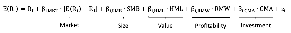
Where, on top of the factors explained in the Three Factor Model:

represents each factor’s coefficient, security ‘s price behavior sensitivity to factor X.

– “Robust Minus Weak”, this introduces the effect of profitability premium into our security or portfolio’s returns.

– “Conservative Minus Aggressive”, this introduces the effect of investment premium into our security or portfolio’s returns.

The Factors

The Five Factor Model uses two new factors to extend the explanation of security or portfolio returns:

• Profitability- this factor captures the historical tendency of more profitable (robust) firms to produce higher returns than less profitable (weak) ones. It is called “Robust Minus Weak” (RMW), since it is calculated as the difference in return between portfolios that have robust company stocks and portfolios that have weak company stocks over a certain period. Profitability can be measured in various ways, but in this case is measured as the ratio between company’s operating income and its equity book value, as appears in its balance sheet. The equity book value serves as a proxy to for the total capital invested in the firm. Relating a firm’s operating profit with its equity book value shows us how efficiently is uses its equity capital to generate profits. Profitable firms and efficient firms and should be rewarded by investors over time.
  
• Investment- this factor captures the historical tendency of companies with lower levels of investment growth (conservative) to produce higher returns than companies with higher levels of investment growth (aggressive). It is called “Conservative Minus Aggressive” (CMA), since it is calculated as the difference in return between portfolios that have conservative companies and portfolios that have aggressive companies over a certain period. Asset growth is typically measured as the percentage annual change in the book value of a company’s assets, as appears in its balance sheet. The book value of a company’s assets changes over time due to various investing activity, depreciation of existing assets and other actions.
  
  A lower growth in total assets implies a cautious approach to expansion, possibly indicating the management’s focus on operational efficiency, higher profitability or risk aversion. A higher growth in total assets implies an expansive investment strategy which can involve significant reinvestment of earnings into the business and the making of investments in assets and means of production. This includes the entering to new markets or developing new products- activities that bear higher levels of risk.
  
  It comes to mind that the investment factor contradicts with the size factor, that suggests that smaller companies tend to show higher returns than large companies. The reason for that may be that small companies are expected to invest more aggressively than large and firmly-based companies. However, a company’s investment behavior is independent of its size. There isn’t a clear link between firm size and its investment behavior. Furthermore, the investment factor relates to a firm’s investment behavior relative to its existing assets and not market capitalization.
  
  A company’s investment strategy is affected by its cash flow levels, its existing leverage, growth objectives, risk tolerance and projections of future market demand. It is also affected by external forces such as industry dynamics and competitive pressures, economic environment and government policies, among other factors.

Conclusion

As we’ve seen so far, since the end of the 19th century, many theories have been trying to explain security return behavior and provide a framework for creating efficient security portfolios. Basically, they all try to make some sense in a complex system of plentiful data and interconnected forces. The challenge still remains today, but there is no doubt- artificial intelligence and machine learning will allow us to move forward and understand the capital markets much better.

Psychological Biases

There is a plethora of psychological factors that stem from our biology and psyche, and negatively influence our portfolio management. These biases stem from each our internal processes, our interpretation of reality and the various shortcuts our mind makes, in order to be able to process all this information. They all lead to irrational decisions.

According to Jose Luiz Barros Fernandes, Juan Ignacio Pena and Benjamin Miranda Tabak, who published a paper titled “Behavioral Finance and Estimation of Risk in Stochastic Portfolio Optimization”^◆ in 2009, these influences can be divided into two groups: Cognitive Biases and Emotional Biases.

• Cognitive Biases- these are basically systematic errors in thinking that occur when we process and interpret information in our environment, leading to skewed judgments and irrational decisions. They stem from the brain’s attempt to simplify information processing. For simplifying the world around us, our brain uses Heuristics, which are basically mental shortcuts. According to the researchers, better information and advice can often correct them.
  
• Emotional Biases- these are interferences to our thinking that stem from feelings and emotions, such as intuition, rather than conscious reasoning. Emotional biases can cloud rational thinking and decision making. According to the researchers, they are hard to correct. It was shown that people whose emotional reaction to monetary gains and losses was more intense on both the positive and negative side, exhibited significantly worse trading performance.

It is important for all investors to identify and understand at least their most prominent biases, in order to tackle them and make better investment decisions. I will now mention some prominent cognitive and emotional biases that influence all investors and affect their results. However, there are well over a hundred identified and documented biases.

Cognitive Biases

1. Confirmation Bias- the natural human tendency to seek or emphasize information that confirms their existing beliefs or theses. Investors are often overconfident because they tend to give their attention to information that appears to confirm the decisions they have already made. 
   
2. Conservatism Bias- the tendency to cling to existing beliefs and underweight new information.
   
3. Anchoring Bias- this is the tendency to rely too heavily on, or anchor to, one piece of information when making a decision, usually the first piece of information acquired. For example, many investors base their decisions on the current share price relative to its trading history.
   
4. Hindsight Bias- hindsight bias is a tendency to see beneficial past events as predictable and bad events as not predictable. Hindsight bias is a dangerous state of mind as it clouds an investor’s objectivity in assessing past investment decisions and inhibits their ability to learn from past mistakes.
   
5. Illusion of Control- the tendency to overestimate one’s ability to control his environment.
   
6. Information Bias- the tendency to put effort in evaluating information even when it is useless in understanding a problem or issue. Investors are bombarded with useless information every day and it is difficult to filter through it to focus on information that is relevant.
   
7. The Dunning-Kruger Effect- this describes the tendency of people to underestimate their own incapability. The people with the least knowledge tend to feel the most confident and show the highest gap between ability and perception. Most new active retail investors experience this effect.
   
8. Base Rate Fallacy- the tendency to ignore general, statistical information in favor of specific, anecdotal information.
   
9. Oversimplification Tendency- individuals prefer simple explanation over more complex ones, even when the simplicity misrepresents the nuances and complexities of a situation. in seeking to understand complex matters humans tend to want clear and simple explanations. Many investment mistakes are made when people oversimplify uncertain or complex matters.
   
10. Neglect of Probability- the tendency to ignore or over/underestimate uncertainties in decision making. This often leads to an underestimation of significant risks, as people disregard rare or uncertain events.
    
11. Representative Heuristic- the tendency to classify new information based on past experiences or stereotypes. People often assume that if something looks like a member of a certain group, it must be a part of that group as well. This may lead to snap, inaccurate judgments due to a situation’s few similarities to an earlier matter.
    
12. Gambler’s Fallacy- this is the belief that if something happens more frequently than normal during a given period, it will happen less frequently in the future, or vice versa. In other words, this is the tendency to believe that future probabilities are altered by past events, when in reality they are independent. Like when gamblers believe they are on a winning streak, even though each event is independent.
    
13. The Law of Small Numbers- the tendency to draw broad conclusions from a sample that is too small in size to make an educated decision. This may cause investors to make generalizations about future security performance based on a short period of monitoring or a small amount of data, which can be misleading.
    
14. Limited Attention Span- humans are constrained by what economist and psychologist Herbert Simon called Bounded Rationality. This theory states that people make decisions based on the limited knowledge they were able to accumulate and their limited ability to concentrate over time. Instead of making the most efficient decision, they’ll make what looks like the most satisfactory decision. Because of these limitations, investors tend to rely on information that is available, easily accessible or attention-grabbing.
    
15. Recency Bias- the tendency to overemphasize the importance of recent events or the latest information we possess when estimating future events. Recency bias often misleads us to believe that recent events can give us an indication of how the future will unfold^◆.

Emotional Biases

1. Overconfidence- investors experience overconfidence in two ways: overconfidence in the quality of their information, and overconfidence in their ability to act on said information at the right time for maximum gain. Studies show that overconfident traders trade more frequently and fail to appropriately diversify their portfolios.
   
2. Loss Aversion- as Daniel Kahneman and Amos Tversky shown in their Prospect Theory, this is the tendency for people to strongly prefer avoiding losses than obtaining equivalent gains. This effect suggests that the pain of losing is psychologically about twice as powerful as the pleasure of gaining. It can lead to poor and irrational investment decisions, whereby investors refuse to sell loss-making investments in the hope of making their money back.
   
   The loss-aversion tendency breaks one of the cardinal rules of investing regarding the opportunity cost: all past decisions are sunk costs and a decision to retain or sell an existing investment must be measured against its opportunity cost, or the other investment opportunities available at each moment.
   
3. The Endowment Effect- this term is closely related to loss aversion. It occurs when people place a higher value on an asset that they own than on an identical asset that they do not own. This means that individuals are likely to demand more to give up an object than they would be willing to pay to acquire it, if they didn’t already own it. This effect shows that ownership can influence the perception of value, leading to potential irrational decisions.
   
4. Incentive-Caused Bias- this is the power that rewards and incentives can have on human behavior. This bias refers to the tendency of individuals to think and act in ways that are aligned with their incentives, often leading to biased decisions and behaviors. This bias can lead individuals to act in ways that serve their personal interest, sometimes at the expense of ethics, rationality or the interests of others.
   
5. Bandwagon Effect (or groupthink, “herd mentality”)- this describes gaining comfort in something because many other people do (or believe) the same. Following the crowd.
   
6. Restraint Bias- the tendency to overestimate one’s ability to show restraint in the face of temptation. Oftentimes, investing creates temptations to make impulsive, irrational trades and many investors fall for it.
   
7. Cognitive Dissonance- this is the mental discomfort individuals experience when they hold two or more contradictory beliefs, ideas or values. To reduce this dissonance, individuals may change their beliefs or justify their behaviors, often through rationalization or denial. This manifests in investing when we make a decision that doesn’t align with our initial analysis or beliefs.
   
8. Familiarity Bias- the tendency to favor familiar or well-known investment opportunity. this leads to an avoidance of anything outside one’s comfort zone. It also brings investors to prefer well-known brands or domestic securities. It often leads to lack of diversification.
   
9. Mood Bias- the tendency of one’s current emotional state or mood to influence his perception in decision making. When experiencing mood bias, individuals may interpret information, make predictions or take actions that are consistent with their current mood, rather than based on objective analysis. This can lead to inconsistent investment decisions, such as over-optimism when our mood is positive, and vice versa.
   
10. Status Quo Bias- the tendency to prefer things to stay the same. Resistance to change. The current condition is taken as a reference point for measuring investment success, and this can cause investors to be unwilling to change their position based on new information. This can lead to suboptimal decision making, as people might stick with subpar options or resist beneficial innovations simply because they represent a departure from what they know and find familiar.
    
11. Regret Aversion- people tend to avoid making decisions that could lead to regret in the future, often leading to overly cautious behavior or decision paralysis. People fear the feeling of regret and avoid it as much as possible, and will sometimes go illogical lengths to avoid having to own the feeling of regret. This bias severely impacts financial decisions, career choices and personal growth opportunities.
    
12. Trend Chasing- this is the tendency of making investment decisions based on recent trends in performance rather than on a comprehensive analysis. Trend chasing is driven by a combination of recency bias and FOMO, leading investors to jump onto the bandwagon of recent success without a solid base for their decisions. If we identify a trend, it’s likely that the market identified and exploited it long before us. 
    
13. Positive Bias of Past Performance Memory- investors’ memories for past performance are positively biased. They overemphasize positive outcomes from past decisions while forgetting or underemphasizing negative outcomes. These positive memory biases are associated with overconfidence and trading frequency, and can lead to an unrealistic assessment of one’s investing skills and potentially to overconfidence. A possible method for reducing overconfidence and trading frequency is exposing investors to their true past returns^◆.
    
14. The Disposition Effect- the tendency to sell assets that have increased in value and hold assets that have dropped in value. Rational investment thinking dictates the continuous analysis of all relevant information in order to make a decision. This effect is driven by a combination of loss aversion and regret aversion, and can lead to suboptimal investment decisions.

The following diagram describes many cognitive and emotional biases and provides some context to each (click to enlarge):

The Portfolio

Basically, we want to create the most efficient portfolio given our goals and constraints. Since we have imperfect information about both the past, present and the future, we seek to include, in our portfolio, securities that we project, to the best of our ability, will show the highest return for any given risk. For this, we often to do the following:

1. Project Returns- project each security’s return. We create an estimation of what we are expecting to receive from getting exposure to a security or asset class.
2. Define and Measure Risk- choose a risk metric and use it to measure our security and portfolios’ risks. Since we can never be sure of future outcomes, we need to choose a method that best fits our preferences and world views.
3. Interrelated Security Analysis- perform comparative analysis of security pairs and combine those that work well with each other. This means we will choose securities that we project will be exposed to different sources of risk, and that their return behavior will be as independent as possible from each other.

Basically, our security portfolio is our position, our total sensitivity to factors and changes in the various states in our environment. In the capital markets, we get compensated for taking risk, in the form of a risk premium, which is return. This comes to incentivize people and organizations to save, think and create positions that will direct resources to where they may be needed in the economy. This uncertainty in anyone’s ability to fully understand the economy and society’s needs, leaves room for people to continuously try to outsmart each other and enhance the resource distribution system in return for financial gain.

In this section, I will first discuss the process of portfolio creation and maintenance, explore how we measure portfolio return and then elaborate on how we measure total portfolio performance, meaning its return in relation to its risk, through some prominent single-index performance measures. I will then conclude this text with a discussion about portfolio investment strategies, which are divided into two sections: portfolio creation methodologies and portfolio management strategies.

Creating a Portfolio

Creating and managing a portfolio is performed “from top to bottom”, by first understanding the investment goals and then formulating a strategy, that results in the creation of a portfolio. Every portfolio is then constantly monitored and rebalanced as necessary. There are 6 basic steps for managing a portfolio over its lifetime:

1. Setting investment objectives- we begin the process of portfolio management by getting a deep understanding of the entity or person whose funds are being managed. We need to understand their goals with investing their capital and their risk tolerance.
   
   • Understanding the investor’s risk tolerance- we achieve this by asking the investor various questions with quantifiable answers. For example, it is customary to ask how much % loss they are willing to take before breaking their position, or grading their risk tolerance. We then use this information to put the investor in the appropriate “box” of risk tolerance. We use this “box” in every step of the portfolio management process and make sure to keep our actions in line with the investor’s risk preferences.
     
2. Establishing an investment policy- at this stage we determine the asset allocation based on the investor’s goals and risk tolerance group. We need to decide how to distribute our investor’s capital over the different asset classes and take into consideration any constraints or restrictions imposed by the investor. At this stage, we usually consider client and regulatory constraints, together with tax and accounting issues.
   
3. Formulating portfolio strategy- at this stage we select a portfolio strategy that is consistent with the investment objectives and policy we prepared. Portfolio strategies can be either active or passive, as discussed above.
   
4. Constructing the portfolio- once we selected our investment strategy, it’s time to physically create the portfolio. We need to research and select the specific assets to include in the portfolio with the goal of creating an efficient portfolio, meaning a portfolio that is projected offer the best return for a given level of risk. We can use any theory or methodology we can think of, such as those I elaborated on in this text.
   
5. Measuring and evaluating investment performance- this includes the calculation our portfolio’s realized return over some time interval and understanding its origins. In this process we do the following:
   
   • Measure returns.
   • Understand the sources of our portfolio’s return: by security, industry and risk exposure.
   • Measure the benchmark’s return and risk and compare with our portfolio, to see whether our management added value by outperforming the benchmark.
   • Understand portfolio performance- whether the manager added value by skill or luck. This is done using single-index performance measures and performance attribution models. We will discuss these concepts in the next part of this text.
     
6. Periodic rebalancing and maintenance- every once in a while, either in predetermined intervals or after major changes in the markets, the portfolio manager “prunes” the portfolio, as with time the different assets change in price, which changes their portfolio weights. Rebalancing is done by selling the winners and buying the losers to keep in line with our original asset allocation. It is thus a contrarian approach to investing.

Measuring Portfolio Return

Measuring a portfolio’s return involves determining how much value the portfolio has gained or lost over a specific period, both in absolute monetary terms and relative percentage terms. This includes both capital gains and any yield generated by the assets in the portfolio. The total return of a portfolio during a given period can be expressed as the sum of these two elements:

1. Capital gains/losses- this is the difference between the portfolio’s market value at the end of the period and its market value at the beginning. The portfolio’s market value is measured as a sum of the market values of its individual assets.
   
2. Yield- this includes all distributions made from the portfolio’s assets during the period, such as dividends or bond coupon payments.

Approaches to Measuring Return

There are two main methods to calculate a portfolio’s return: Periodic Return and Total Return.

1. Periodic Return (Index Creation)- this method calculates each asset’s return over a specific period, averages them based on the portfolio’s weighting, and updates an index at regular intervals.
   
   Periodic return compounds returns over time, with each period building on the previous one. It smooths fluctuations in asset prices and accounts for volatility drag, where high volatility reduces cumulative returns due to the lower geometric average compared to the simple average.
   
   While periodic return tracks performance over time, it doesn’t directly translate into cash flows, as it reflects unrealized returns until the position is settled. Common metrics used in this method include simple and logarithmic returns, mean return, compound return, and IRR.
   
2. Total Return (Start to End)- this method calculates the final value of each security relative to its initial value, adding the yield generated during the period. It creates a weighted average of these returns for the total portfolio, assuming straight-line growth without compounding.
   
   Total return measures the actual cash flow the investor receives and is ideal for calculating realized returns. This method often uses simple return, compound return, and IRR metrics. Unlike periodic return, it doesn’t account for the effects of volatility, which can sometimes result in a higher return compared to periodic compounding.

At the bottom line, we use periodic return to understand the trajectory of a portfolio’s performance path, and total return to understand the actual cash flows from an investment.

Common Return Metrics

There are several key metrics used to measure returns, each suited to different goals and time horizons:

1. Simple (Arithmetic) Returns- this is the simplest way to measure a portfolio’s return. It is often used for quick snapshots over a single period and represents actual cash flows. It measures the return relative to the initial value, either in percentage or absolute monetary terms.
   
   Simple returns ignore the time value of money and investor contributions. They calculate the difference between the portfolio’s initial and current value, adding any yield. This method is best for short periods where the time value of money is less significant. However, simple returns are path-dependent, as they only consider the first and last prices, ignoring fluctuations in between. This can lead to an inaccurate reflection of the portfolio’s performance over multiple periods.
   
   The portfolio’s simple (arithmetic) return, relative to its initial value in per-cent terms, is calculated as follows:
   
   
   
   And its simple return in absolute, monetary terms is calculated as follow
   
   
   
   Where:
   
   is the portfolio’s ending market value, at time , as measured by the combined values of its constituent securities. This is roughly the cash we will get if we sold the portfolio’s assets today.
   
   is the portfolio’s beginning market value, at an earlier time , the starting period of return measurement.
   
   includes any dividend or bond coupon payments, called “distributions”, made to the investor during the period. This is the yield.
   
2. Logarithmic (Continuously Compounded) Returns- while arithmetic returns are useful for single-period analysis and represent actual cash flows, they can be misleading when analyzing an asset’s performance over multiple periods, especially when compounding is involved.
   
   Logarithmic returns, or continuously compounded returns, offer a more accurate reflection of performance over time because they incorporate the effects of compounding. They capture the entire return path, which is essential for accurately reflecting continuous compounding. Therefore, they are ideal for multi-period analysis, especially when significant volatility is present. Unlike simple returns, logarithmic returns can be summed across periods to accurately capture compounding effects, making them ideal for statistical analysis.
   
   Logarithmic returns are calculated using the natural logarithm of the ending value divided by the beginning value. They are symmetrical around zero, meaning they properly account for percentage changes over multiple periods. For example, a increase followed by a decrease will bring logarithmic returns back to the original value, unlike arithmetic returns, which would show a lower figure.
   
   Logarithmic returns, also known as continuously compounded returns, are calculated using the natural logarithm of the ending value (), divided by the beginning value (). It looks like this:
   
   
   
   Converting Between Simple and Logarithmic Returns
   Converting between simple returns and log returns is important since log returns naturally handle compounding, while simple returns do not. The first one focuses on performance analysis that depends on the performance path and the second one focuses on actual cash and the bottom line. We are able to move between these two return types, depending on our needs:
   
   • From Simple to Log Returns- we can convert a simple return into a log return using the following formula:
     
     
     This conversion allows us to analyze the return properly, in a way that reflects compounding effects over time, which is important for long-term performance analysis.
     
   • From Log to Simple Returns– conversely, if we want to convert a log return back into a simple return, the formula is:
     
     
     
     This conversion is useful when we want to express returns in a simpler form that represent actual cash flow, and is easier to interpret over shorter periods.
     
3. Mean Returns- to understand a portfolio’s average performance over time, we often use the mean. Depending on the data and context, we use different types of means:
   
   • Arithmetic Mean (Simple Average)- this is the most straightforward application, that provides a basic idea of how the portfolio performed on average during a time frame. It is calculated by summing the periodic returns and dividing them by the number of periods. It is sensitive to outliers and is best used for short-term performance or yield-generating portfolios, as it shows the average yield per period. It looks like this:
     
     
     
     Where each represents a periodic return.
     
     The arithmetic mean is sensitive to outliers, as a single very high or low value can significantly impact the result.
     
     It’s best used for short-term performance evaluation or for yield-generating portfolio, as it can clearly show us the average yield per period.
     
   • Geometric Mean- this mean calculates the product of the returns, making it ideal for measuring compounded returns. It is more suitable for long-term investment performance, as it accounts for growth volatility and compounding effects. It looks like this:
     
     
     When used in portfolio management to calculate average return, based on arithmetic returns that do not take compounding into account, we often adjust it by adding 1 to each return value and then subtract 1 from the result. It looks like this:
     
     
     The adjustment accounts for compounding, where each growth rate influences cumulative growth. The geometric mean is unsuitable for sets with zeros or negative numbers, but adjusting to relative terms provides an accurate reflection of portfolio growth over multiple periods.
     
     The geometric mean is best used for assessing long-term investment performance as it accounts for the compounding of returns over time. It also accurately reflects the impact of growth volatility on the portfolio’s value.
     
   • Harmonic Mean- this is the “reciprocal of an arithmetic mean of the reciprocals of the numbers” in a set. Useful for averaging ratios, the harmonic mean is robust to outliers. It’s particularly valuable when comparing fractions or ratios between elements. However, it is undefined if any values are zero. It looks like this:
     
     
     The harmonic mean is undefined with zero values but is ideal for averaging ratios and handling significant outliers.
     
     So to conclude, we often use the geometric mean to calculate returns with reinvestment, and the arithmetic mean for when we don’t reinvest capital into the portfolio. We will mainly use the harmonic mean for a better representation of ratios.
     
4. Compound Annual Growth Rate (CAGR)– sometimes we need a single, smooth growth rate over a period, especially for comparing multiple portfolios. The Compound Annual Growth Rate (CAGR) provides this by calculating the average annual return, smoothing out volatility. Given the start and end values, and the number of periods, the CAGR calculates the average growth rate over the entire period.
   
   Given the start value, end value and the number of periods, the CAGR calculates the average periodic growth rate. For portfolio management, it results in a portfolio’s average periodic return. It looks like this:
   
   
   
   Where:
   
   is the value at the end of the period.
   
   is the value at the start of the period.
   
   is the number of periods, usually years, in our timeframe.
   
   CAGR is often used to compare portfolios and project future returns, assuming past behavior remains constant. However, it assumes reinvestment and ignores significant cash inflows or outflows, so it may not always reflect the actual growth of investments with periodic cash changes.
   
5. Internal Rate of Return (IRR)- for longer periods and for portfolios that experience regular contributions and distributions, a better way to measure the return of a living portfolio. This is where the Internal Rate of Return (IRR) calculation comes in, resulting in a single annual per-cent figure. For the IRR, we note the initial investment amount, changes in our portfolio’s value and any periodic cash flows, that we treat as net distributions (distributions minus contributions) on a monthly/quarterly/annual basis. We input this data on a timeline.
   
   An explanation of IRR and its calculation is found above under the Definitions section. IRR calculates the portfolio’s annual return, including the time value of money, periodic distributions, and reinvestment. It is ideal for long-term periods with cash inflows and outflows.
   
   These return calculations generate gross figures, meaning they exclude any costs associated with creating and managing the portfolio or any tax payments on yield or capital gains. If we included these expenses we would get a net figure to the investor.
   
6. Annualizing Returns- whether we are using simple returns, logarithmic returns, or more complex metrics like IRR, our measurement can be for either shorter or longer periods than an exact year. There is often a need to annualize these figures for easier comparison across different time periods. Annualization transforms returns calculated over shorter or longer periods into annual terms, allowing you to compare investments on a consistent basis.
   
   For returns and other figures that do not involve compounding, meaning reinvestment of gains and the time value of money, we use a straightforward adjustment. Our annualized value looks like this:
   
   For returns and other figures where compounding is involved, a different formula is applied to reflect the effect of reinvestment. We do it in the following way:
   
   Where:
   
   is our investment return on a yearly basis.
   
   is the return we calculated for our period of interest.
   
   is the 1-year representation using our time periods: 365 or 252 (trading) days or 12 months.
   
   is the length of the period on which we have return data, in the same representation: days, weeks, months etc.
   
   When , our investment period is shorter than one year, so we are scaling up the return. When , our investment period is longer than a year, so we are scaling down the return. Both actions will transform our periodic return figure to reflect an annual period.
   
   Annualizing returns converts partial or multi-year returns into an equivalent annual figure, allowing for easier comparison across investments. It reflects the rate of return if sustained over a full year but does not represent actual gains or losses.

When measuring portfolio performance, we consider both return and risk. Risk means the return is not guaranteed, and more risk increases the chance of things going wrong. The goal is to create an efficient portfolio, maximizing return for each unit of risk. I’ll now discuss how we measure this efficiency.

Measuring Portfolio Risk

We never focus only on portfolio returns. As I mentioned above, return is granted to investors for taking risk in the capital markets and enhancing the resource distribution system.

The following measures quantify a portfolio’s risk:

• Variance and Standard Deviation- this is the basic measure of risk in portfolio management. It stems from the thinking that people would prefer small and steady increments in return over large swings. As defined in the Statistical Analysis Definitions sections, variance measures the dispersion of a set of data points around their mean value. In portfolio management, these data points are the periodic returns. A higher variance indicates a wider dispersion of returns, implying a higher risk since the portfolio’s performance could deviate significantly from the expected return.
  
  Standard deviation is the square root of variance. It represents the average deviation of a data point from the mean that is expressed as the same units as the data, and is therefore more easily understood and used.
  
  Both variance and standard deviation assume that returns are normally distributed, and only take the first two moments of the distribution of returns: the mean and the variance, into account. They ignore the skewness and kurtosis that return distribution functions often show. They therefore do not fully capture the risk of extreme events, or the represent the true risk of a security or portfolio.
  
• Downside Deviation- this is a measure for the dispersion of returns that fall below a threshold. This risk measure was discussed under the Post-Modern Portfolio Theory (PMPT) above. For reference, it looks like this:
  
  
  Where:
  
  is the threshold: the Minimum Accepted periodic Return for the relevant timeframe.
  
• Maximum Drawdown- on a historical examination of our portfolio’s value, this is the worst loss that we would have experienced if our portfolio was created at the peak and sold at the trough within the specified timeframe. To calculate the maximum drawdown, we identify our portfolio’s highest value and the following lowest value before a new peak is formed, and then we calculate the difference in per-cent between the lowest point and the previous peak. This measure comes to quantify the “worst case scenario” of a loss, as happened in the past.
  
• Value at Risk (VaR)- VaR focuses on the potential downside risk of a portfolio. It estimates the maximum loss a portfolio could face in a given period with a certain confidence level, under normal market conditions. It is a statistical measure used to assess a portfolio’s possible future loss, as visible in the at Risk term.
  
  VaR is expressed in three parts: the amount of potential loss, the time period over which the risk is assessed, and the confidence level in our assessment. For example, VaR can indicate that our portfolio has chance of losing at least or over the next timeframe. This means that under normal market conditions, there is a confidence level that the portfolio’s loss will not exceed or over the next timeframe.
  
  This statistic has several advantages, as it is a single number expressed in the units of its data and is therefore easily interpreted. It fits all cases when there is a good understanding about the distribution of a random variable.
  
  Var’s limitations include lack of ability to predict the maximum loss beyond the specified minimum, severe underestimation of extreme events and high sensitivity to the method used for calculation. It’s also sensitive to the assumptions made about market conditions and future portfolio return distribution.
  
  While standard deviation, as a measure of risk, measures how much returns vary over time, VaR measures the minimum potential loss that a portfolio might experience over a given period of time.
  
  VaR is calculated using one of three methods:
  
  • Historical Simulation- in this method, we look back at our portfolio’s historical returns and use them to estimate future losses, so this method does not impose a specific distribution for portfolio returns. However, it assumes that the future mirrors of the past, which is a false assumption that we face in varying severities in portfolio management.
    
    We implement the Historical VaR method through the following steps:
    
    • Collect data- collect the past periodic returns of the portfolio’s securities over a certain timeframe.
    • Calculate portfolio return- calculate the portfolio’s past periodic returns.
    • Sort by value- order these returns in a list from worst losses to highest gains. This is basically our portfolio’s past return histogram.
    • Determine the confidence level- this represents the probability that the loss will not exceed the VaR value.
    • Identify the percentile that corresponds to the desired confidence level- a 95% confidence level means that we are looking at the worst 5% of outcomes. We look for the periodic return found at the 5th percentile of past periodic returns from the worst end. This specific return indicates the maximum expected loss over the specified time horizon with a 95% confidence level. This is the maximum expected loss, not the maximum possible loss.
    • Convert per-cent to cash- convert the identified percentile return into a monetary value, representing potential loss. This is usually done by applying the return to the current value of the portfolio.
      
  • Variance-Covariance (Parametric VaR)- this method assumes that portfolio returns are normally distributed and calculates VaR using its mean expected return, variance and the covariance of its constituent securities. This method is computationally efficient but the reliance on the assumption of a normal distribution of returns often creates a distorted view of risk. It looks like this:
    
    
    Where:
    
    is the Z-score corresponding to the desired confidence level.
    
    this is the vector of security weights in the portfolio, and is its transposed vector.
    
    is the covariance matrix of our securities past periodic returns.
    
    The term stands for our portfolio’s standard deviation of past periodic returns.
    
    this is the time horizon in the same period granularity used in for the analysis.
    
    This method basically applies the Z-score to the portfolio’s standard deviation, in order to estimate how far from the mean the portfolio’s return might deviate within that confidence level. The assumption of a normal distribution is what allows us to use the Z-score to begin with.
    
    We implement the Parametric VaR method through the following steps:
    • Collect data- collect the past periodic returns of the portfolio’s securities over a certain timeframe.
    • Calculate portfolio return- calculate the portfolio’s past periodic returns and its standard deviation, through the covariance matrix of its constituent securities and their weights.
    • Determine the confidence level- this confidence level corresponds to a Z-score, which indicates how many standard deviations away from the mean the cut-off point is.
    • Calculate the Z-score- based on the selected confidence level, determine the Z-score using standard Z-score tables. For example, a 95% confidence level corresponds to a Z-score of about 1.645.
    • Compute Parametric VaR- multiply the Z-score by the portfolio standard deviation of past periodic returns and then adjust for the forward-looking timeframe for VaR calculation. The result of this operation is the maximum amount of cash the the portfolio is expected to lose for the given confidence level over the specified forward-looking timeframe. This is the maximum expected loss, not the maximum possible loss.
      
  • Monte Carlo Simulation- while the historical and parametric VaR calculations rely on past data, the Monte Carlo Simulation method for VaR calculation rely on forward-looking assumptions and statistical modelling. It uses algorithms to simulate a wide range of possible future outcomes and calculates the potential losses that could occur in each scenario.
    
    This method can accomodate various return distributions. It is flexible and better captures the risk of extreme market movements. However, it is computationally intensive and carries severe model risk due to its reliance on a model and its assumptions.
    
    We implement the Monte Carlo Simulation VaR method through the following steps:
    • Define the model- we begin by defining the mathematical model that describes the portfolio securities’ future behavior. This includes determining the factors that effect security prices and how they are expected to behave. These models often involve stochastic processes to capture the randomness in market movements.
    • Simulate random outcomes- we use the model we defined to simulate a large number of possible scenarios for how the market conditions might evolve over the specified timeframe. This occurs by applying random variations to the model’s parameters, reflecting the uncertainty of the capital markets.
    • Calculate portfolio return in each scenario- we calculate the return that results in each simulated scenario, as we take into account how each security’s price is affected by the simulated market conditions.
    • Aggregate results- after we made a large number of scenarios and kept the results of each, we combine them into a distribution of periodic portfolio returns. This distribution represents the wide range of possible outcomes for our portfolio, based on our model and assumptions.
    • Determine the VaR- now that we created a distribution of periodic returns, we determine the confidence level and calculate the VaR.
      
• Conditional Value at Risk (CVaR, Expected Shortfall)- this risk metric quantifies the potential extreme losses, found at the tail of the distribution of past periodic returns. While VaR estimates the maximum potential loss at a specific confidence level, CVaR provides an average of the losses that occur beyond the VaR Threshold, making it more sensitive to the shape of the tail of the distribution of returns. It is therefore considered to be a more comprehensive risk measure than VaR.
  
  CVaR calculates the expected loss over a specified timeframe, the loss that is worse than the VaR threshold. This means that it considers the severity of extreme, tail outcomes, and not just the threshold of these outcomes.
  
  We can illustrate CVaR visually like this:
  
  
  ^{Source: CERN Pension Fund.}
  
  We implement the CVaR method through the following steps:
  • Calculate VaR- as per the steps mentioned above.
  • Calculate average loss- the mean potential loss from all outcomes that are worse than the VaR.
    
• Conditional Drawdown at Risk (CDaR)- this risk metric is used to assess a portfolio’s potential downside risk. It measures the the expected maximum drawdown that could occur with a given level of confidence over a specified time period. Unlike VaR that focuses on the standard deviation of portfolio returns, and is thus limited to single-period returns, this approach quantifies the risk of significant declines, even through multiple consecutive periods.
  
  These are the steps for calculating CDaR:
  • Collect data- collect the past periodic returns of the portfolio’s securities over a certain timeframe.
  • Calculate portfolio return- calculate the portfolio’s past periodic returns and its standard deviation, through the covariance matrix of its constituent securities and their weights.
  • Identify drawdowns- look back at the portfolio’s historical periodic return data and identify the drawdowns, which as defined above, are the largest declines from peak to trough before a new peak is formed. We start at the beginning of our time-series, which is a dataset of our portfolio’s past periodic returns ordered by date, and move forward into the future. Every time we pass a drawdown, we identify it and tag its per-cent value in a list.
  • Sort drawdowns- arrange the drawdowns in a list from largest to smallest, showing the worst drawdowns at the top.
  • Determine the confidence level- this is the threshold for CDaR, the percentile of worst drawdowns to focus on. A higher confidence level will focus on more severe but less probable drawdowns.
  • Compute CDaR- calculate the average of the worst drawdowns beyond the selected confidence level threshold, the percentile. This average represents the CDaR, providing an expected value for the worst-case drawdown scenarios.
    
• Maximum Daily Loss- this risk measure is used to assess the potential loss a portfolio could face in a single day, based on either historical data or simulations.
  
  When we calculate the maximum daily loss by directly using historical data, we get a simple outcome: this maximum daily outcome will equal the worst performing loss our portfolio has experienced in the past, under its current structure.
  
  Calculating this measure by using a statistical model, such as VaR, brings a more sophisticated approach to quantifying this possible loss, that now also takes the distribution of past periodic returns into account. Either way, the result is the expected maximum loss our portfolio could endure within one day.
  
• Portfolio Turnover- this risk measure reflects the frequency of trading actions in a portfolio during a timeframe, typically a year. A high turnover indicates a more active management style that leads to high transaction costs and possible capital gains tax implications. The portfolio turnover measure calculates the percentage of assets in the portfolio that have been replaced or traded within the timeframe. It looks like this:
  
  
  Where:
  
  stands for the total cash value of securities bought during the timeframe.
  
  stands for the total cash value of securities sold during the timeframe. We take the minimum value of the two, but some versions of this measure add them up.
  
  this is the average value of the portfolio’s securities. It is calculated by taking the average of the value at the end of the period and the value at the beginning of the period.
  
  A low turnover, such as bellow 20% annually, suggests a buy-and-hold strategy, that results in lower transaction costs and potentially lower tax liabilities on capital gains. A high turnover, such as above 100%, indicates active trading and perhaps even recurring attempts at making short-term gains.

Understanding Portfolio Performance

In order to accurately analyze a portfolio’s performance, we must look both at the return it achieved and the risk that was involved with this return. We have many measures for connecting our portfolio’s return and the risk embedded in its exposure to events in the environment. They are mostly structured as fractions, where an expression that represents return is situated in the numerator, and an expression that represents risk is situated in the denominator, creating a ratio for return for risk.

There are two tasks for understanding portfolio performance: first, when analyzing our portfolio’s performance ex-post, we need to understand whether the return our portfolio generated duly compensates us for the risk we’ve taken. Second, when analyzing our portfolio’s performance ex-ante, we need to know whether the projected return compensates us for the risk we are about to take.

Generally, since different measures take different information into account, it’s best to use several methods in order to get a clearer picture of our position. The most common portfolio performance measures are the following:

• Sharpe Ratio^◆– devised by the economist William Sharpe in 1966 and called “the reward-to-variability ratio”, this ratio is achieved by dividing a portfolio’s excess return over a risk-free asset, meaning its return over the market’s risk-free interest rate, by the standard deviation of its periodic returns over the timeframe. It basically quantifies our portfolio’s risk premium to the actual risk it takes, and can tell us if we got a good deal. It looks like this:
  
  
  Where:
  is the standard deviation of our portfolio’s returns, usually daily over a period such a year.
  
  The Sharpe Ratio shows our portfolio’s excess return per unit of risk, as measured by the standard deviation of its periodic returns. It indicates how much risky return our portfolio earned for the amount of total risk it assumed. Therefore, a higher Sharpe ratio is better. Like other ratios, this ratio lets us plan security selection and compare between different securities and portfolios.
  
• Treynor Ratio- this ratio was introduced by Jack L. Treynor and called “the reward-to-volatility ratio”. It is achieved by dividing a portfolio’s risk premium by its market beta. It looks like this:
  
  
  Where:
  is our portfolio’s market beta, it’s sensitivity of returns to market movements, calculated on past periodic (daily/weekly/monthly) returns over a period of several years, depending on our holding horizon.
  
  The Treynor Ratio is a risk-adjusted measurement of return based on our portfolio’s exposure to market risk. It indicates how much return our portfolio earned for the market risk it assumed. Therefore, a higher Treynor ratio is better.
  
• Sortino Ratio- this was discussed under the Post-Modern Portfolio Theory (PMPT) above. For reference, it looks like this:
  
  
  
• Jensen’s Alpha- developed by Michael Jensen in the 1960s, this is a portfolio performance measure that represents the actual return above or below the portfolio’s expected return as predicted by the CAPM model. This means it measures the difference of the actual portfolio return and what should have been achieved by the level of systematic risk we took on ourselves. It is therefore an Alpha that takes risk into account. It looks like this:
  
  
  Where:
  is our portfolio’s return over a timeframe.
  
  is our the risk-free rate of return over the same timeframe.
  
  is the portfolio’s total exposure to market risk as measured by the slope of the least-squares line between the market and portfolio periodic returns over several years, depending on our expected holding period.
  
  is the return of the market portfolio over a timeframe. This portfolio is theoretical due to the technical difficulty in getting exposure to all the securities in the market, so in practice it is replaced by the country’s main market capitalization-weighted index such as the S&P 500.
  
  is the market risk premium- the general excess returns investors got for taking the extra risk of exposure to risky assets.
  
  If this measure shows a positive value, it suggests that our portfolio has earned an excess return over what the CAPM had predicted, indicating superior management performance that takes both return and risk into account. If it shows a negative alpha, it indicates that our portfolio had underperformed the CAPM’s prediction, suggesting inferior management performance. An alpha of zero indicates our portfolio’s return is consistent with the CAPM’s, or any other model used to forecast return, predicts.
  
• Appraisal Ratio- this is a single-index performance evaluation measure used to quantify a portfolio’s return over a timeframe per unit of risk. It is calculated by dividing the portfolio’s Jensen’s alpha as defined above, by the standard deviation of this alpha. It looks like this:
  
  
  Where:
  is Jensen’s Alpha.
  
  is the standard deviation of Jensen’s alpha, as analyzed ex-post on past periodic data over a timeframe.
  
  In the Appraisal ratio, we basically calculate the difference between a portfolio’s periodic returns and subtract from those the corresponding benchmark return. We then measure the standard deviation of this set of differences. lower indicates consistent excess returns and is preferred, as it hints at skill.
  
  Like many other portfolio performance ratios that place performance in the numerator and risk in the denominator, the higher the appraisal ratio- the better.
  
• Information Ratio (IR)- this ratio is similar to the Appraisal Ratio, but differs in that it takes the simple alpha into account- the one that only measures portfolio return above a benchmark. The ratio then compares this difference with the volatility of its periodic differences. It looks like this:
  
  
  Where:
  is our benchmark’s return over a timeframe.
  
  is the Tracking Error: the standard deviation of the differences between the pairs of periodic portfolio and benchmark returns.
  
  Like the Appraisal Ratio, this measure gives another angle to quantifying our level of investment skill and our ability to generate excess returns relative to a relevant benchmark. It also helps us identify any consistency in our portfolio’s performance.
  
• Tracking Error- this measures the standard deviation of the differences between a portfolio’s periodic returns and its comparison benchmark. It is used to assess our performance in replicating the performance of a benchmark index, if this is our goal.
  
  Basically, this measures how well our portfolio was able to mimic a benchmark without major distortions: a low tracking error means the portfolio moves similarly to the benchmark, and a high tracking error means the portfolio is more disconnected from the benchmark. It looks like this:
  
  
  Where:
  is our portfolio’s return in period .
  
  is the benchmark’s return over period .
  
  is the total number of periods over which the tracking error is calculated.
  
• R-Squared ()- as described in the Statistical Analysis Definitions section above, R-squared quantifies the fit of a regression model to its data. This statistical measure is integral to regression analysis, and serves a pivotal role in portfolio management when applied as a single-index performance measure. In this context, R-squared evaluates the extent to which movements in a portfolio’s value can be attributed to value fluctuations in a benchmark index.
  
  R-squared can take any value between 0 and 1, with a high value indicating a strong correlation with the index, which implies that a signifiant proportion of the portfolio’s performance is driven by market movements. A low R-squared value suggests that our portfolio is largely independent of market movements and that other factors, possibly our own actions, have a more substantial impact.
  
  R-squared helps us evaluate the effectiveness of our portfolio management strategy in relation to market movements, that happen independently of any action we take.
  
• The Modigliani Risk-Adjusted Performance Measure ()^◆– this metric was developed by Franco Modigliani and Leah Modigliani in 1997, as they wanted to create a portfolio performance measure that is easier to interpret than the Sharpe Ratio. They came up with the , which just like the Sharpe Ratio is a risk-adjusted performance measure, but the expressed in percentage points. This difference makes it easier to understand. It shows how well the investor is rewarded for taking a certain amount of risk, relative to the market portfolio’s return and the risk free rate. It looks like this:
  
  
  Where:
  this is our portfolio’s Sharpe Ratio.
  
  these are the market portfolio and our portfolio’s standard deviation of past periodic returns over the timeframe, respectively.
  
  stands for portfolio return over the same timeframe.
  
  , as we have seen, stands for the risk free rate over the timeframe.
  
  The basically multiplies the portfolio’s Sharpe Ratio with the standard deviation of the market portfolio, an action that converts this risk-adjusted excess return into the same risk units as the market portfolio, which then allows for a direct comparison of our portfolio’s performance with that of the market.
  
  An higher than the market portfolio’s return indicates that our portfolio has shown a better risk-adjusted performance and vice versa.
  
• Sterling Ratio- this performance metric was proposed in 1981 by Deane Sterling Jones, as a way to evaluate the performance of commodities trading advisors (CTAs) and hedge funds, focusing on how well these managers handled downside risk relative to their returns.
  
  It compares a portfolio’s Compound Annual Growth Rate (CAGR), its average annual return, with a risk figure represented by the average annual drawdown over a timeframe.
  
  It looks like this:
  
  
  Where:
  is the return CAGR our portfolio has generated over the specified time timeframe.
  
  this measures the maximum drawdown in each year of our historical analysis timeframe and then calculates their average. As explained above in Measuring Portfolio Risk, maximum drawdown is the largest peak-to-trough decline in the portfolio’s value during a timeframe, before a new peak is formed, measured in per-cent. This figure represents the worst loss a portfolio have endured in the relevant timeframe.
  
  this is a per-cent value that some versions of the Sterling Ratio use in order to represent the risk free rate. During this ratio’s conception, the risk free rate was 10%, and so this figure stuck and used by practitioners today^◆. It serves to increase the denominator and thus reduce the ratio. The larger the risk free rate, the smaller the ratio will be. We take the absolute value of the difference between the average annual MDD and the constant.
  
• Calmar Ratio- this performance metric was proposed by Terry Young in 1991. It is similar to the Sterling Ratio, in that it uses a portfolio’s Compound Annual Growth Rate (CAGR) to represent returns, but this time the risk measure is the maximum drawdown over the timeframe, based on past data. It is usually used for evaluating the performance of strategies that are prone to high volatility, such as the case when using leverage.
  
  It looks like this:
  
  
  Where:
  while the Sterling Ratio measures an average, annual maximum drawdown, the Calmar Ratio uses the maximum drawdown during the entire analysis timeframe, and here lies the difference between the two ratios. It is common to calculate the Calmar ratio’s maximum drawdown over a period of three years, but the exact timeframe can change as needed. We take the absolute value of this decline.
  
  Unlike other ratios, this performance metric puts emphasis on the maximum drawdown as the primary measure of risk, making it relevant for portfolios where large drawdowns are a primary concern. A higher Calmar ratio indicates a more favorable past risk-adjusted return, as the position generated higher returns per unit of risk, as measured by the maximum drawdown.
  
• Upside Potential Ratio- a ratio of periodic returns above a threshold and the volatility of those below it, this risk measure was discussed under the Post-Modern Portfolio Theory (PMPT) above. For reference, it looks like this:
  
  
  Where:
  is the threshold: the Minimum Accepted periodic Return for the relevant timeframe.
  
• Omega Ratio^◆◆– this portfolio performance measure gives us a more complete view of our portfolio’s performance, as it takes in our portfolio’s full periodic return distribution over a timeframe and uses it to assess its return-risk profile. This means that the Omega ratio takes all the distribution moments into account, and not just mean and variance like the previously mentioned performance measures, and gives us a clearer picture. For this reason, it is a better and more useful metric for portfolios that do not exhibit normal return distributions.
  
  The Omega ratio is calculated by dividing the total gain instances, over a certain return threshold, by the the total loss instances, meaning periodic returns were below that threshold, over a timeframe.
  
  The ratio is created by dividing two integrals, which are mathematical tools that measure the area under a function line. While in math, integrals sum up infinitesimally small pieces to calculate an area under a curve, in return distributions they serve a simpler purpose. Distributions are basically a function form of histograms that count periodic figures. In a histogram setting, integrals just stand for counting: we count how many periods our portfolio returned higher than the threshold, and how many periods it returned lower than the threshold. Then we create a ratio by dividing the two. It looks like this:
  
  
  Where:
  The integrals calculate the areas under the curve of the cumulative distribution function. The numerator calculates the potential gains above the threshold and the denominator calculates the potential losses.
  
  is the threshold return, often considered the minimum required return. This can either be the risk free rate or some return target the investor seeks to achieve.
  
  is the cumulative distribution function of returns, which gives the probability that the return r is less than or equal to a certain value. This is a general function that represents the probability that the random variable, in this case the portfolio’s return, will take a value less than or equal to r.
  
  A higher Omega ratio indicates a more favorable reward-risk profile, as there is a larger area above (to the right of) the threshold relative to the area below it (to the left of the threshold).
  
  The following figure can help make things clearer. It shows a hypothetical return distribution that happens to look like a Normal distribution, shows the threshold and the areas to its right and left:
  
  
  ^{Source: investexcel.net.}
  
  In reality, this distribution can take any shape and form, as the ratio focuses on the area below the function line, which was created by actual, past periodic return figures.
  
  This ratio has some unique advantages: as mentioned, it provides a more complete picture of our portfolio’s historical and therefore projected return behavior, but also offers flexibility in that it lets us set the threshold as per our needs. This means it lets us incorporate our own preferences. It also does’t assume a normal distribution of returns, which is often a false assumption in security analysis. Like all statistical measures, this ratio focuses on the past and requires enough trading data in order to create a return distribution.

Investment Strategies

As we saw, we first create portfolios and then manage them over time. These two stages involve two different groups of investment strategies: the first is portfolio creation methodologies, which focuses on the creation part, and then the portfolio management strategies, which focuses on the ongoing decision-making and tactical adjustments within the portfolio, based on the changing market conditions.

Both investment strategies can belong to one of two overarching approaches to investing: active and passive. As defined in the Definitions chapter above, active investing means that we periodically analyze the market and make investment decisions regarding our portfolio. Passive investing means, that we create a portfolio that mimics a market index and let it be for the long run. In both approaches we periodically rebalance our holdings to maintain our desired exposure to risk.

Portfolio Creation Methodologies

Portfolio creation methodologies focus on how portfolios are initially created, emphasizing the principles guiding the selection and weighting of securities. They involve the planning and execution of an optimal investment portfolio based on our current knowledge of the market and the investor’s preferences. In practice, we combine several methodologies and end up with a set of securities and their weighting in the portfolio in a way that best fits a set of requirements.

Each of the following portfolio creation methodologies can guide us when we come to allocate our capital between securities and asset classes.

Classical Asset Allocation- this has been the prevalent portfolio construction strategy since the Modern Portfolio Theory (MPT). It introduced diversification by dividing the investor’s capital between stocks and bonds in a certain proportion, based on his risk appetite. Risk-seeking investors will require higher exposure to equities at the expense of fixed-income securities, and vice versa. 60/40 means 60% equities and 40% bonds. Equities are considered a more risky asset type than fixed income, since they are situated lower at a company’s cash flow waterfall and they are the last to receive payment.

After deciding on the suitable equity-to-bond ratio, investors select specific asset classes within equities and bonds to further diversify their portfolio. They can then choose individual securities or get exposure through ETFs. Periodic rebalancing is required to keep the required proportions, as market movements will change this ratio over time.

Market Capitalization-Weighted Portfolio (Value Weighting)- under this strategy, we assign weights to securities of asset classes based on their market capitalization, which is the total value of their equity. This will cause larger companies to get a bigger proportion of the portfolio. This is the method used in market-cap weighted indexes such as the S&P 500 or the NASDAQ 100. The rationale under this approach is that larger companies have a more significant economic impact.

Equally-Weighted Portfolio- this is the easiest and most straight forward portfolio creation strategy. Under this strategy, each security or asset class is allocated the same percentage of the portfolio’s total value. This transparent and simple strategy effectively gives investors a higher exposure to smaller companies than what would have been under the market-cap weighted strategy. Due to its creation style, its return pattern deviates from that of the most widely-used market-cap weighted indexes that represent whole markets, making it harder to benchmark and compare return-risk tradeoff.

Mean-Variance Optimization for Portfolio Creation- as per the ideas of the Modern Portfolio Theory (MPT), we use the mean-variance optimization to better understand the various securities we think of adding to our portfolio, and how they interact. We adjust the securities and their weights in our portfolio in order to achieve a certain projected return and risk. This portfolio is created by finding the security weights that minimize the volatility of the entire portfolio’s projected return or maximize projected return for a given level of risk, based on the constituent securities’ past return variance and their correlations with each other.

Volatility-Weighted Portfolio- we can create portfolios by weighting each security or asset class inversely to its volatility. This method results in higher allocations to less risky securities, and vice versa for more risky securities. Each security or asset class’ weight in the portfolio is determined as:

Where:

is the standard deviation (or any risk measure) of security or asset class .

represents the sum of all our portfolio’s securities or asset classes’ inverted risk measures. A security’s weight is basically the ratio between its inverted risk and the total inverted risk of all securities in the portfolio.

Risk Parity- this strategy creates lower-risk portfolios and focuses on allocating risk equally among the portfolio’s securities, not capital. This often involves leveraging lower-risk assets to ensure that each asset class contributes equally to the portfolio’s overall risk. Risk Parity is different from volatility-weighted portfolio creation in that Risk Parity takes into account the entire distribution of a security or asset class’ risk, whereas the volatility-weighted approach only takes into account each security’s standalone risk.

Volatility Targeting- this strategy is executed by first setting a required level of portfolio risk, as measured by volatility, and then creating the portfolio. The portfolio creation is done using securities that together are projected to show the required level of volatility regardless of market conditions.

Factor Investing- also called Smart Beta, this investment strategy seeks to create a diversified portfolio of securities that are exposed to different risk factors, or in other words, are sensitive to different events in the environment. It is best if the securities’ return behaviors are as little correlated to each other as possible.

Core-Satellite Investing- just as suggested by the Treynor-Black model, under the core-satellite strategy investors create a passive, long-term strategy as the core of their investment strategy, and apply an active, short-term tactical asset allocation to try and achieve short-term gains. The allocate their capital between these two strategies.

Direct Indexing- this strategy involves the creation of a personalized portfolio that replicates an index by directly purchasing the underlying securities, leaving room for customization and security selection. This strategy also introduces tax benefits.

Thematic Investing- this strategy involves identifying and investing in companies that we project will benefit from macro-level trends over the long-term.

Sector Allocation- this strategy involves distributing investments across different sectors of the economy, achieving both reasonable diversification and leaving room for investor judgement.

Preference-Based Investing- this involves creating a portfolio based on investor preferences, such as various ethical considerations like Environment, Society and Governance (ESG), impact investing or the avoidance of areas the investor seeks to avoid.

Geography-Focused- this strategy involves the diversification of securities across some desired geographies.

Income-Focused- this strategy aims at generating a steady income of cash return from the asset ownership, typically through dividend payments for stocks or interest payments from bonds. It allows investors to enjoy the fruit of their investments without the need to sell them.

Duration-Targeting in Fixed Income- a type of interest rate immunization, this strategy involves managing the sensitivity of the bonds in a portfolio to interest rate changes by adjusting the bonds’ duration, which is the weighted average time it will take to receive all principle + interest payments on a bond. For fixed interest rate bonds, higher duration means higher sensitivity to changes in interest rates.

Liquidity Management- when investors have their liquidity requirements in mind when creating their portfolios, they will make sure to keep a suitable proportion of liquid securities that will allow them to convert them to cash as needed. They can build the yielding part of the portfolio to match their required expenses.

Tax Efficiency- tax-efficient investing brings tax considerations into portfolio creation. It aims at minimizing tax liabilities and maximizing after-tax returns.

Portfolio Management Strategies

Portfolio management strategies determine how a portfolio is maintained over time, in order to optimize its results for its goals. Once a portfolio is created, these strategies involve decisions about when to buy or sell securities, how long to hold them and when to rebalance the portfolio. Some portfolio creation strategies can be extended and used for management as well.

I will briefly discuss several prominent portfolio management strategies:

Value Investing- this is an investment strategy that focuses on examining an asset’s economic value and current price. The investor generates some kind of valuation for the asset and compares that to the asset’s current price, whether in public markets or in a private offering. If they conclude that the price is lower than the asset’s value, they should get a long exposure by buying the asset and wait for the price to align with their valuation. This dynamic basically offers a premium for being smarter than the rest, which means having the ability to read reality better, identify value where others are blind to it, and act. A renowned economist named Benjamin Graham pioneered this portfolio management strategy since the 1930s with his book Security Analysis (1934) and later The Intelligent Investor (1949).

Growth Investing- this investment strategy focuses on companies that show signs of above average growth compared to their industry or the overall market, even if their share price appears expensive in terms of metrics like the Price-to-Earnings (P/E) ratio. Growth investors are usually more concerned with a company’s future potential earnings growth than its current valuation. They expect to earn a return when the company grows faster than the market anticipates and prices.

Buy and Hold- this is a type of long-term, passive portfolio management strategy, whereby investors get ownership of securities and hold them for an extended period of time, regardless of market fluctuations. This strategy is based on the belief that in the long-term, societies and economies grow and this translates to a satisfactory expected annual return. This belief is based on solid grounds, as the US S&P 500 has shown to provide an annual return of about 9.9% per annum including dividends, and about 6.6% per annum when adjusting to inflation, between Jan-1928 and Dec-2023^◆. Buy and Hold also involves lower transaction costs and tax efficiencies due to the few trades.

Momentum- this is an active portfolio management strategy that is based on the tendency of securities to continue a trend. Momentum investors buy securities trending upwards and sell short securities trending downwards, profiting in case these trends persist.

Dollar-Cost Averaging- this portfolio management strategy relates to the management of time, rather than securities. It involves making regular investments of a fixed amount into the portfolio, regardless of the securities’ price. The aim behind this strategy is to diversify the investor’s exposure to his assets through time, reducing the impact of volatility on the overall security ownership. This makes us buy more securities when their prices are low and fewer securities when their prices are high. We implement this strategy when we don’t try to time the market, meaning we don’t put thought on the exact time of security purchase.

Capital Preservation- this portfolio management strategy focuses on protecting the original invested capital from loss or erosion, prioritizing the safety of the principal over the pursuit of high returns. This involves both protection from inflation and capital loss. This strategy often involves buying stable securities such as government bonds or treasury bills, and is often used by investors that are risk-averse, or those with a short-term investment horizon.

Inflation Protection- this portfolio management strategy focuses on safeguarding the purchasing power of capital against the eroding effects of inflation. Rather than prioritizing nominal returns, the goal is to ensure that the real value of the investment keeps pace with or exceeds inflation over time. This strategy typically involves investing in assets such as Treasury Inflation-Protected Securities (TIPS), real estate, commodities like gold, or equities, which have historically provided protection against rising prices. Inflation protection is crucial for long-term investors seeking to maintain or grow their wealth in real terms, especially in inflationary environments.

Income- this portfolio management strategy focuses on generating a steady stream of income from investments, often prioritizing consistent cash flow over capital appreciation. The goal is to produce regular payments in the form of interest, dividends, or rental income, making it especially popular among retirees or investors seeking stable, predictable returns. Common investments in an income strategy include dividend-paying stocks, bonds, real-estate investment trusts (REITs), and other income-generating assets. While the focus is on income generation, this strategy still considers the preservation of capital, though some risk may be taken to achieve higher income yields.

Making Money

Ok then, so how do we make money investing?

In the previous sections of this paper we explored the various portfolio management theories, the numerous psychological biases all investors face and also explained more about the essence of a portfolio. In this section I will connect everything together, and link information with return. This section provides what I see as solid advice for portfolio management.

Starting with the sources of return. Basically, as the Capital Asset Pricing Model (CAPM) identified, investors can earn a return in two ways:

1. Systematic Risk Exposure- investors get a systematic return for exposing their capital to risks stemming from the system itself (a.k.a systematic risks). The return arising from exposing our capital to these risks is the capital allocation system’s way of incentivising its participants to operate it, by providing it with capital, resulting in overall economic growth. The more efficient the system is in absorbing information and reflecting it in prices, the more prominent the part of systematic risk in an investor’s returns, at the expense of idiosyncratic risk.
   
   This source of return represents a more passive style of investing, intended for a holding period of at least several months. It only requires the investor to identify the systematic risks he wants to get exposed to, employ his capital and wait patiently for the economy to grow.
   
   Most investors do not identify the systematic risks they are exposed to, and settle for creating this exposure by investing in main market benchmarks such as the S&P 500 or Nasdaq 100. They gain exposure to these indexes by buying Exchange Traded Funds (ETFs) or mutual funds that facilitate the concurrent exposure to dozens or hundreds of securities.
   
   For example, it is customary to consider various credit, market, and operational risks into this category, as they stem from the economic system itself. The illiquidity premium of alternative investments can also be considered a systematic market risk that bears systematic return.
   
   There is no room for alpha in this source of return, only beta- the sensitivity of our portfolio to various systematic risks. In literature, some sources simplify matters by defining alpha as any return above what a model predicts. However, this view suggests that any excess return above the model’s forecast, arises merely from the model’s partial ability to capture systematic risk sources. This interpretation of alpha is overly simplistic and vague, as it fails to reflect the true essence of alpha- investment skill.

2. Idiosyncratic Risk Exposure- classical investment theories like Modern Portfolio Theory suggest that investors should pursue maximum diversification and avoid idiosyncratic risks. However, these theories rely on a stringent set of assumptions, such as market efficiency, market equilibrium and zero transaction costs, and following them fully would bring failure. The over-diversification they promote deprives the market its most important asset- active investors. Without active participants, the system would lose its capacity for thought and implode. Capital allocation would collapse.
   
   In reality, investors can get consistent idiosyncratic return by continuously gathering and processing information about specific companies or sectors. They earn this return for knowing something others don’t and acting faster to establish efficient positions. By conducting thorough analysis, investors create positions and anticipate that, over time, the market will discover the information and adjust prices accordingly, generating profits.
   
   When we make decisions based on smart analysis, we embed the information we gathered into asset prices. This not only provides capital to the system, but also signals areas in the economy that we believe there is unmet demand. Our actions provide a little capital to the areas we discovered, increasing asset valuations and making it easier for companies to obtain financing, in order to create supply in the medium to long-term. If our theses are correct and other investors follow, our positions will increase in value and we will make profits.
   
   The consistent use of information for achieving better return for a given risk can be referred to as Information Alpha. This is the capital allocation system’s way of incentivizing its participants to collect, process and use data and information to understand the economy’s true needs. Active investors bring wisdom into the market and this is the source of their compensation, whether by identifying undervalued companies or spotting bubbles and selling short. This understanding is reflected in asset prices, affecting the distribution of resources in the economy. It’s the return investors get for making the system smarter.
   
   While classical theories assume that markets are efficient in absorbing information, in reality they are not (see discussion about the Efficient Market Hypothesis above)^◆. Efficiency is achieved gradually, over time, through the actions of millions of active investors who collect information and apply thought to their investment decisions. Markets are therefore not perfectly efficient, and equilibrium is a theoretical concept that represents an area, rather than a single point. In his book “The Alchemy of Finance”, George Soros illustrates how investors’ psychological biases influence their decision making, depriving the markets from the ability to reach equilibrium.
   
   Idiosyncratic risk exposure represents a more active style of investing, requiring investors to actively seek information, think critically and act quickly. This is also often exemplified by stories of investors who observe their immediate environment and make investment decisions based on the information they gather. For example, the story of Peter Lynch and how he decided to buy Dunkin’ Donuts shares^◆.
   
   Since markets are not perfectly efficient, there is still a lot of information that can be used to gain a return by helping them become a little more efficient. Capital markets are filled with random noise, psychological biases, asymmetrical information, transaction costs and also credit incentives, among other types of disruptions that affect the efficient flow of information. As markets become more efficient, it becomes harder to gain returns from using information, and expected returns tend to diminish. Nevertheless, even though the system is not perfect in absorbing marginal information, it can still generally operate effectively.
   
   Investors not just give, but also receive information from the market all the time. In order to generate information alpha, the market, as represented by a significant number of investors, needs to agree with our thesis and pour capital in the direction of our position. If our assumptions are correct, we can choose to realize our profits as we see fit. When the opposite happens, we need to reexamine our assumptions and perhaps change our theses, and consequently modify our position.

The more an investor is able to understand the components of the systematic risk he is exposed to, the better off he is in any case. The more he is able to collect, analyze and model information to form an educated investment thesis, the more information alpha he will be able to generate by exposing himself to idiosyncratic risk.

The problem with both sources of returns, but especially information alpha, is psychological biases that affect all human investors. All investors face difficulty in converting their thought into action, without them being distorted by psychology.

Use Information to Drive Performance

While existing theories focus on understanding systematic risk and leveraging it to generate returns, this chapter emphasizes the active side of investing, using information to achieve information alpha.

In active investing, our goal is to understand the economic environment better than others. By forming theses, assigning probabilities to various scenarios, and positioning ourselves accordingly, we aim to anticipate market movements before the broader market reaches the same conclusions. In doing so, we can profit when prices adjust to reflect the information we have acted on.

Information is constantly being created and disseminated around us, but it does not spread equally or simultaneously across the market. Sophisticated investors are often the first to form theses, gather supporting data and establish positions. These investors rely on the gradual dissemination of information to the broader market, which influences the demand and prices for the securities they own as it disseminates. Typically, information reaches investors in order of their sophistication, with retail investors often reacting last.

To understand how information drives prices, consider the example of an asset bubble. While only a small fraction of assets follow this extreme trajectory, the mechanisms at play reveal the relationship between information, psychological biases and price behavior.

George Soros, in his book “The Alchemy of Finance”, describes this process as a “boom-bust cycle” where psychological biases amplify price movements. Historical examples include the Dot-Com Bubble of the late 1990s, the rise, fall and subsequent rise of Cryptocurrencies, the phenomenon of meme stocks and many more. These events illustrate how markets react to both solid information and irrational exuberance.

The following chart illustrates the trajectory of an asset bubble, showing how prices rise sharply due to reasons unrelated to fundamental value and eventually fall just as dramatically when the bubble bursts:

What this chart tells us:

• Proximity to the Origin and the Value of Information- the closer we are to the origin, the more valuable and scarce the information is. Sophisticated and patient investors are the first ones to act on this limited information, as no quick gains are usually promised at this period. In the Stealth Phase and Awareness Phase, investment decisions are made by firm hypothesis testing and rational decision making based on fundamental analysis. Investors establish their positions early and wait for a sufficiently large mass of capital to find its way to the same assets, by other investors that reach the same conclusions.

• Information Embedding Over Time- as time passes, more information is disseminated in the market and becomes incorporated into asset prices. This is evident during the Awareness Phase, where initial price increases are often followed by minor reductions as early investors realize profits. The asset may experience small corrections due to psychological biases, market noise and imperfect information dissemination.
  
• Formation of Bubbles Due to Psychological Biases- bubbles, or “boom-bust” dynamics, often occur after prolonged periods of gains and especially with increased participation of less sophisticated investors. In the Mania Phase, investment decisions become heavily influenced by psychological biases such as fear of missing out (FOMO), over-optimism, herd mentality, the bandwagon effect and familiarity bias. These biases lead to sharp price increases that are disconnected from reasonable assessments of economic value, often neglecting the ever-existing influence of competition. Eventually, as steep as the boom was, the bust is just as steep, and the bubble bursts in the Blow-Off Phase.
  
  This is when most investors often lose interest and look for opportunities for quick gains somewhere else.

For these reasons, prudent investing is hard on two fronts:

• Early Opportunity Identification- identifying opportunities during the Stealth Phase requires extensive research and the ability to form theses before the majority of investors.
  
• Maintaining Conviction- holding positions during downturns is difficult, especially when market beta exposure leads to losses. Continuous validation of investment theses through updated analysis is critical.

Opportunistic investing is risky on two fronts:

• Diminishing Returns- late-stage investors face reduced upside as the opportunity becomes widely known. Psychological biases further inflate prices, increasing the risk of sharp declines.
  
• Increasing Uncertainty- in the Mania Phase, traditional risk measures underestimate true risk due to reliance on past data and an inability to quantify biases.

How Holding Periods Drive Performance

The investment holding period fundamentally influences the sources and nature of returns. In the short term, investing resembles a zero-sum game: one investor’s gain equates to another’s loss (or missed profit). This period is fraught with psychological biases and random noise, largely reflecting the shifting sentiments and opinions of investors.

By contrast, long-term investing transcends zero-sum dynamics. Here, returns are grounded in the true economic growth that capital markets nurture, allowing more investors to benefit collectively. Long-term performance is rooted in genuine analysis and a real understanding of economic fundamentals, whereas the short term often relies on “technical analysis”, which is essentially an attempt to anticipate the behavior of other investors.

In the short-term, the market gets what it wants. In the long-term, it gets what it needs.

Diversify

As we discussed in the Modern Portfolio Theory section above, it is important to emphasize that for both sources of return, diversification is crucial for better expected results. It is a gift from the system that should be used by all investors. While investors seeking exposure to various systematic risks are diversified by definition, investors seeking information alpha through idiosyncratic risk exposure should still seek to diversify across multiple assets, even though obtaining information alpha gets harder for the more assets we have. Nonetheless, diversification enables more resilient portfolios, balancing specific insights with broader market exposure.

For maximum effect, the securities should have as little connection to each other as possible, often measured by the correlation of their past periodic returns. The closer the figure is to 0 in absolute value, the stronger the effect of diversification. It is always best to understand why the securities’ return behavior is not connected, and not rely just on correlation analysis, which can be random and time-dependent.

We should diversify our holdings based on their true nature, aiming to create portfolios that are balanced in their exposure to various risk factors. Relying on traditional distinctions of asset classes and recommended allocation proportions no longer guarantees robust portfolios. The old 60/40 rule for equities and bonds is insufficient for achieving true diversification. Instead, we must analyze each security’s exposure to risk and build portfolios with balanced exposures that align with our expectations about future events and market conditions.

In reality, all investors’ capacity for pursuing information alpha is limited. Most investors, which are able to gather just little information, would be wise to employ the Treynor-Black Model and create a “core-satellite” portfolio. They should combine a strategic allocation to systematic risks (80% of capital) with a tactical allocation (20%) based on their information and analysis about the economy’s unmet needs. However this is not marked in stone- the more sure they are in their information and assumptions, the more they should allocate to the “satellite”.

Diversification will not be able to match the possible return-to-risk characteristic of true information that indicates a change that the market has yet to discover, especially in the short-term. In cases of strong conviction, where unique insights reveal undervalued opportunities, some investors may choose to reduce diversification to amplify returns, accepting the higher idiosyncratic risk while systematic risk exposure remains largely unchanged. However, the more we really feel certain about our investment thesis, the more we should stop and remember that we may be affected by psychological biases.

Weight Securities

What about portfolio weighting? How do we make the decision on how much capital to allocate to each portfolio component?

Every action of investing starts with choosing the securities we want to use in order to materialize our investment thesis, and then their weighting. As we discussed above, various theories have risen over time, trying to bring sense into this bias-tainted decision. None was able to provide a single solution, since such solution doesn’t exist.

In theory, we should only weight our securities based on our certainty about their future performance trajectory, as we envision in our theses. We can order them in a list by their expected return-to-risk ratio, discard those that fall below a threshold and then try to guess the probability of each scenario happening. The securities that embody the highest expected return to risk should get the most allocation. We can describe the general task as follows:

Where:

this is security ‘s expected return over our expected investment period.

is security ‘s expected risk, as expressed either in standard deviation or any other measure of risk, over our expected investment period.

The ratio can also be converted to “risk premium” terms by subtracting the expected risk-free rate from the expected return, creating what is also known as the Sharpe Ratio.

is the minimum value of the ratio we expect to achieve.

is the probability of all that happening in reality.

We can easily see that 3 out of 3 of these variables are forward looking, which makes it impossible to get them right. Basically, weighting is the focal point of our beliefs about the future, which can never be 100% predicted: in the short-term, our finely-granular data is infected with random noise. In the long-term, it is affected by many factors, some more difficult than others to measure. Since we can never know for certain where our analysis and assumptions and the market will meet, we try to make educated guesses. And this is where psychological biases get in.

Therefore, since the aforementioned task is based in prediction and serves as a means to divide our capital between securities, we would be smart to take a different approach. It is much simpler and smarter to just allocate our capital equally between the various securities, and use diversification to control our weighting. For example, for a portfolio of 10 securities, we can choose 2 that are expected to be exposed to similar risks, instead of 1.

Measure Risk Correctly

Our goal in measuring portfolio risk is to quantify the potential capital loss within a specified time interval, at a given confidence level. By understanding this, we can estimate how much capital is at risk under normal market conditions, enabling us to make smarter decisions about our capital exposure and tolerance for risk.

As surprising as it may be, most investors do not understand the true risk of their investment actions. Most investors rely on standard deviation of returns, which is the square root of return variance, as a representation to how much capital they can lose. This measure is both easy to calculate and simple to interpret, as it’s expressed in return percentage terms, reflecting the degree of return fluctuation around the mean return.

Using historical, periodic, simple (not log) returns, the standard deviation indicates how much an asset’s or portfolio’s periodic returns have deviated from the mean return over a given timeframe. A larger standard deviation indicates more spread-out past periodic return occurrences, meaning the asset was more volatile and therefore riskier. Usually, the basic assumption in describing investment risk is that past standard deviation will persist into the foreseeable future, provided there are no material changes in the nature of the underlying business.

In investing, we use simple returns to highlight the actual return an investor can expect in every period, and use a histogram of past periodic returns as a tool to analyze a security’s risk profile. This approach helps transform “uncertainty” into quantifiable “risk” and make solid investment decisions.

However, the standard deviation of returns is often not a good measure for understanding investment risk, leaving investors unable to properly value assets.

First, as it is symmetrical in nature, meaning it measures both profit and loss, the standard deviation is a somewhat inaccurate way of measuring investment risk. In their Prospect Theory, Kahneman and Tversky found that the pain of a loss is stronger than the joy of making profits, but standard deviation treats upside price movements the same as downside price movements.

Second, since standard deviation is a representation of the average distance between each return and the mean, it is sensitive to outliers. Outliers are unusually large or small investment returns that significantly deviate from the typical range. This means that a single outlier can disproportionally inflate the standard deviation, making an asset appear riskier than it may be under typical conditions, that occur in the vast majority of periods. Ignoring these outliers also distorts the true nature of an asset’s risk.

Third and most important, the fact that outliers are inherent to investing brings a more significant issue with standard deviation: it can only mean something if the distribution of past periodic returns is symmetrical around the mean. On top of that, it is most reliable only when our portfolio’s returns follow a normal distribution.

In a normal distribution, the returns are symmetrically distributed around the mean, with skewness and excess kurtosis equal to 0. Only in this case does the Empirical Rule apply and we could draw meaningful probabilities about expected asset price behavior. According to the rule, we can ascertain that 68% of observations will fall within one standard deviation of the mean, 95% within 2 standard deviations and 99.7% within 3 standard deviations.

This rule demonstrates why standard deviation can effectively predict risk under normally distributed returns: it provides clear probabilities that an asset’s returns will stay within these ranges. This bell-shaped distribution gives investors a consistent risk measure.

However, as returns diverge from normality, the Empirical Rule no longer applies, and standard deviation becomes a less reliable measure of actual risk of capital loss. In real markets, it’s common for asset returns to display “fat tails” (positive excess kurtosis), where extreme returns occur more frequently than a normal distribution predicts. This fat-tailed behavior significantly increases the likelihood of significant losses, or tail risk, which standard deviation underestimates.

Actually achieving a normal distribution, or even a symmetrical distribution of returns, is very rare in the world of publicly traded securities. A normal distribution of returns requires us to make various assumptions that do not hold in reality. See the following violations:

1. Independence of returns- returns should be independent both across securities and over time. This means the return of one security should not affect another, and the return in one period should not influence the next period’s return for the same security. However, in reality, securities are interconnected, as information from one asset or market can impact others. Furthermore, returns over time often exhibit autocorrelation, where today’s returns can predict or influence tomorrow’s, contradicting the independence assumption.
   
   Standard deviation assumes that each return is independent, meaning the return of one period or one security does not influence another. If returns are correlated, standard deviation becomes less reliable because past returns can predict future returns, skewing the return distribution.
   
2. Identical distribution- returns should be drawn from the same probability distribution. This assumption also does not hold in reality, as each security and its underlying business mechanism behaves differently.
   
   The requirement for independence of returns, along with identical distribution, forms the assumption of independent, identically distributed (i.i.d.) returns, which is often violated in practice. This dependence and different distributions of returns violate the assumption of i.i.d. returns that is foundational in many financial models.
   
   If returns come from different distributions, standard deviation may under- or overestimate the true volatility. It will only provide an average measure of variability over the sample, which might be misleading if risk changes significantly over time.
   
3. Stationarity- in time series analysis refers to the idea that statistical properties, such as mean and variance, remain constant over time. In financial markets, however, non-stationarity is common, as the variance of actual returns fluctuates with the changing economic conditions. When modeling future returns (such as by assuming past standard deviation will hold), practitioners often encounter heteroskedasticity in the model’s residuals, where the variance of error terms, which are the differences between modeled results and actual results, changes over time. This happens because market volatility shifts, creating volatility clustering, which refers to prolonged times where high-volatility periods follow one another, as do low-volatility periods.
   
   This clustering indicates that the model’s residuals are not constant, which conflicts with the assumption of constant residual variance (homoskedasticity). This reveals that the relationship between predicted and actual returns is unstable. As a result, relying on standard deviation becomes risky, as the assumption that past return volatility will persist does not hold, likely misrepresenting future risk.
   
   In other words, if returns are non-stationary, using standard deviation as a future risk measure is unreliable, since past return behavior does not necessarily persist.
   
4. A sufficient sample size- in statistical analysis, a larger sample size improves reliability. If the sample size is too small, the standard deviation may be heavily influenced by outliers or temporary market conditions, making it less representative of the true volatility. Ideally, we need at least 30 observations to perform robust analysis, but in practice, most investors hold far fewer assets, making statistical predictions about return distribution or risk more uncertain and potentially misleading.
   
   We can use standard deviation with smaller portfolios, but the results may be less reliable and subject to greater variability.

Standard deviation works best when these assumptions hold because, under these conditions, the historical variability is a reliable indicator of future variability. However, When returns are not independent, or when they are drawn from changing distributions, standard deviation loses its predictive power. Since these assumptions rarely hold in real-world markets, portfolios typically do not exhibit normal or symmetrical return distributions. This renders the use of standard deviation inadequate for most investors when assessing risk of loss.

In other words, without normally distributed returns, standard deviation fails to capture a large part of our portfolio’s actual potential for losses in a given time period. This is primarily due to its underestimation of tail risk and the unequal nature of non-symmetrical distributions. As a result, standard deviation misrepresents the portfolio’s true exposure to extreme events, and understates its actual downside potential.

In other words, when an investor uses the standard deviation of returns as the only means of describing risk, his model is too simple and therefore highly biased. He is partially blind, leaving the room for more sophisticated players to fill the gaps in his understanding and take profits out of his flimsy portfolio positioning. This may be what paves the way for investment strategies like value investing, which describes and measures risk differently and thrive in periods of market panic, where opportunities abound. During these periods, all who rely solely on standard deviation of returns are blindsided by worst-case scenarios and leave the market.

To gain a clearer understanding of our true chances of losing money, regardless of the shape of the return distribution, we should consider alternative risk measures. Statistical analysis of past data, such as VaR and the Omega Ratio, offers additional perspectives for quantifying investment risk. These concepts are discussed above in the Measuring Portfolio Risk and Understanding Portfolio Performance sections. However, the correct and wholesome way of understanding investment risk lies in our position’s overall exposure to all that can go wrong. The more sensitive our position is to occasional events, the more risky it is.

Buy Cheap

The concept of “buying cheap” is intuitively relatively understood, but what does it truly mean? Generally, the quality of a deal, the asset being “cheap” or “expensive”, is a measurement of the distance between its price and its value, which is a figure representing all its future economic benefit under reasonable forward-looking assumptions.

Ex-post, in retrospect, we measure the distance between the price we paid for the asset relative to the price it had reached in a later period, representing its value. If the price went up over that time period, we can say we bought it “cheap”. The opposite goes for “buying expensive”, when the asset’s price dropped below our expectation.

Ex-ante, before buying an asset, buying cheap means that according to our information and beliefs, the offered price is below its expected economic value, as we perceive it in our model. This implies that we can enter a position at a price that does not fully reflect all available relevant information, potentially resulting in a future profit. Again, the opposite goes for “buying expensive”.

Either way, “buying cheap” is a time-dependent concept that relies on our ability to discover an asset’s most probable economic value and own the asset for a price beneficial to us: lower than that assessment when we have long exposure to the asset, and higher when we have a short exposure.

The fact that the asset’s price in the market can be different than our assessment stems from the idea that other investors make the same efforts of valuing assets, with varying degrees of success. At the point of investment, our goal is to enter a position that we believe will result in a favorable return trajectory, based on our analysis and insights, which may differ from those of our counterparties.

Understand the Difference Between Value and Price

As discussed in Asset Valuation, there is a material difference between these two key concepts:

• Value- from an economic perspective, value is a subjective assessment of the most probable economic benefits we can derive from owning an asset. It is based on various forward-looking assumptions about factors that are often beyond our control. To estimate an asset’s economic value, we need to create a model, input the relevant information that is available for us, make assumptions about the future, and calculate a number that reflects the combination of all these elements. Since we are dealing with forward-looking assumptions, it is always good to enhance our model with scenario analysis. When used for investment decision making, value is always forward-looking and probabilistic.
  
• Price- this is the actual amount of capital exchanged during the transfer of ownership of an asset. It represents where the forward-looking assumptions of various market participants converge into a single point, resulting in a deal. Price can never truly reflect “true value” because such a definitive value doesn’t exist. Value is in the eyes of the beholder.

At the point of investment, , we must utilize all the information at our disposal and make educated guesses about the future. Other market participants, including the asset’s current owner, are doing the same. Everyone attempts to gather information, process it, model it, and arrive at some notion of “fair value” for the asset. No one can predict the future perfectly, so no one knows exactly what this value truly is. These are all educated estimations.

The investor who can make a good deal is the one who better anticipates the asset’s return trajectory and sets a bid or ask price accordingly. The following illustration may help defining these concepts:

The difference between price and value stems from the markets’ inefficiency in absorbing information. This means that the price will never be equal to value, and that different investors will reach different valuations for the same asset.

The differences in valuations reached by different investors come from each investor’s unique needs, tastes, information and psychological biases. Before buying an asset, we need to assess whether there is material information that the market has yet to incorporate into the price. Using our available information and expertise to formulate reasonable assumptions, we estimate a value that we are comfortable with.

To determine where an asset’s price stands relative to its value, we must first establish a valuation for the asset, then compare the offered price to that estimate. There are various methods to value assets, with the Discounted Cash Flow (DCF) analysis being the most prominent, deep and resource-intensive approach for cash-yielding assets, as discussed in detail in Asset Valuation. However, applying DCF is typically reserved for substantial capital allocations, as it requires significant time and effort, making it less practical for every investment opportunity.

Valuation Shortcuts

While DCF is the most comprehensive way for investors to translate information and analysis into an estimation of value, investors often don’t use it to analyze every cash-yielding investment opportunity. In practice, most investors use valuation ratios as quick, shortcut models that provide us with indications of the distance between price and value, often referred to as “mispricing”.

These ratios typically consist of a price metric divided by a profit measure, and sometimes the other way around. Each ratio represents value by comparing what an investor pays to what he gets.

We calculate valuation ratios by using available information and plugging the relevant figure into the formula, and then adjust them using our own information and expectations. This creates two values for each ratio: market ratio and our own ratio. The distance between them represents differences between our perception of an asset’s value and the market’s expectations. If our ratios are higher than the market’s, this means that we believe the asset is undervalued, “cheap”, and vice versa.

These differences between the derived ratios and our own ratio calculations offer valuable perspectives on how our views differ from market expectations. How do we use our own information and expectations to calculate our own ratios? Using the following methods, from easiest to hardest:

1. Comparison to self- we can compare the business’ current ratios with their past ratios, include any new information that is now available, and try to conclude if relative to its past, the current ratios are a true representation of the asset’s value.
   
2. Comparison to others- we can compare the business’ current ratios with those of its competitors and try to conclude if relative to its peers, the security is undervalued, meaning that its ratios should be higher (and vice versa). We can also compare it to the market as a whole, as represented by a benchmark such as the S&P 500, Nasdaq 100 or the sector index.
   
   It’s important to compare a company’s ratios to similar peers in terms of field of activity, revenue, geographic focus etc., since this will provide a purer comparison. The further a peer is from the company we are examining, the more adjustments we would have to make to close the gaps in their activities, quickly rendering the comparison ineffective.
   
3. Model financial figures- somewhat compromising the idea of quick valuation shortcuts, we can create a quick model for implementing our own assumptions about the asset’s value figure, and plug it into the ratio, and compare our ratio with that of the market’s.

By combining these methods, investors can use valuation ratios to make better decisions, achieving a balance between efficiency and a deeper representation of an asset’s value.

Some prominent valuation ratios include:

1. Price-to-Earnings Ratio (The P/E Ratio)- this is a common metric that compares a company’s current price with its annual earnings (net profit). It can also be expressed on a per-share basis (divided by the number of outstanding shares). It is calculated as:
   
   
   This ratio can be used on an ex-post basis (looking at past 12-month earnings) or an ex-ante basis (using expected earnings for the next 12 months). It represents how much investors are willing to pay for a dollar of earnings.
   
   To interpret its outcome:
   • Lower P/E Ratio may indicate that a stock is undervalued or has lower growth expectations, but it can also reflect market concerns about the company’s future earnings stability or growth potential.
   • Higher P/E Ratio often suggests that investors expect strong future growth or earnings potential, though it can also indicate that the stock is overvalued relative to its current earnings.
     
2. Price-to-Earnings Growth Ratio (the PEG Ratio)- introduced by Mario Farina in 1969^◆, the PEG ratio refines the P/E ratio by incorporating expected earnings growth, bringing the focus of valuation into the future growth of earnings. It is calculated as:
   
   
   It serves as a quick indication of value based on price, earnings and the expected annual growth rate of those earnings. To interpret its outcome:
   • PEG < 1 indicates that the asset may be undervalued relative to the growth prospects we foresee for it. It means that based on the information at our disposal, the actual earnings growth rate will be higher than what others think.
   • PEG = 1 indicates that the asset is fairly valued, and the price is able to capture all available information used to assess future earnings growth.
   • PEG > 1 indicates that the asset may be overvalued relative to the growth prospect we foresee for it. It means that based on the information at our disposal, the actual earnings growth rate will be lower than what others think.
     
3. Price-to-Book Ratio- this ratio compares a business’ market price to its book value:
   
   
   It serves as a quick indication of how reasonable the price is against book value, as calculated by a certified accountant following accountancy rules, representing a company’s net asset value. To interpret its outcome:
   • P/B < 1 indicates that the stock is undervalued, as the market price is less than the company’s net asset value.
   • P/B > 1 indicates that investors expect future growth or intangible assets not reflected on the balance sheet.
     
4. EV/EBITDA- the Enterprise Value (EV) to Earnings Before Interest, Taxes, Depreciation, and Amortization (EBITDA) ratio assesses a business’ value while considering its debt and cash levels. It looks like this:
   
   
   Where Enterprise Value (EV) is equal to + – .
   
   It serves as a quick indication of how reasonable the business’ enterprise value against its annual EBITDA. To interpret its outcome:
   • Lower EV/EBITDA may indicate that the company is undervalued.
   • Higher EV/EBITDA could suggest overvaluation.

While these are the main ratios for a quick indication of value, there are others. They all basically divide the current asset price with some kind of valuation or repeating earnings figure, and they are all used to view the distance between price and value in new angles for a deeper, more accurate picture.

Structure Decision Making

The investment process is basically the same for all investors, but more so for those seeking information alpha. It should be structured and clear in order to stay focused and maintain control of the process:

1. Form an investment thesis- get an idea about a way to make profit and enhance the system. Identify an area where the market has yet to embed information and is unaware of coming demand. This area is usually touched by business mechanisms, such as companies that issue shares, but also through alternative investments.
   
   For example, did we encounter a company that works very well, sells very well, and the market has yet to discover? Or a sector that is about to enjoy higher demand, and require investments in assets for value creation?
   
2. Gather information- in this stage, the goal is to collect both qualitative and quantitative data to support or refute our thesis. While earnings reports and revenue projections provide hard figures, understanding management’s track record, industry dynamics, and potential regulatory impacts are equally important qualitative factors. Alternative data sources are also great, since they are harder to find, more local and less used. Keep in mind that gathering relevant data doesn’t only mean more data but better data that directly supports or refutes your thesis.
   
3. Model the data- here we create a model that turns the data and information we collected into knowledge and provide actionable insight. For example, investors that seek fundamental analysis might lean on valuation models such as discounted cash flow (DCF) analysis to estimate a company’s intrinsic value. Investors can even explore machine learning models for identifying patterns in historical price data. The goal here is to bring order into the data and get knowledge out of it, to support or refute our thesis.
   
   Models offer the advantage of scenario and sensitivity testing. Once we have a solid model we can examine the different outcomes of our investment decisions based on things that happen in our environment. This is where factor models come in. Models also force us to make assumptions where needed, such as the general lifespan of our position and other forward-looking assessments.
   
   At this stage we should understand the sources of our expected return: what needs to happen in the market and the economy in order for us to generate a return based on our thesis. What systematic risk factors will our portfolio be exposed to? What kind of idiosyncratic risk?
   
4. Identify securities- find assets that are exposed to the area of the economy we identified. Sort them by order of how they fit in achieving our desired exposure to the area. The purer exposure, meaning a high relation to the area, the better. Keep in mind the effect of the connection between the securities’ return behavior on diversification, as the ones that are more disconnected offer a better diversifying effect.
   
   We should focus on businesses we can understand, so we can be sure we got things right. We need to be able to understand if and how the businesses will be able to create more supply and meet the rising demand quick enough, while the competition is still not biting into profit margins and therefore valuations.
   
   Peter Lynch recommends we try to understand a business’ story. The story should be simple, such that we can explain to a 10 year-old in less than 2 minutes, and he would get it. The more complex the story is, the more probable it is that it falls apart. The simple ideas are the ones that have the highest chances of succeeding. The goal for a good business management is to correctly identify a problem and solve it in an efficient manner.
   
5. Create a position- choose the financial or alternative assets that create the most efficient portfolio that captures our beliefs. They should be of sufficient quantity to achieve diversification, while still maintaining a sufficient exposure to the area of the economy we have identified. This is also where the decision on security weightings comes in. It’s usually best to keep things simple and explainable.
   
   At this stage we should understand our true exposure to risk, meaning our chance to lose a specific amount of capital in a given period.
   
6. Validate thesis- monitor the position and constantly seek new information that arrives and embeds into the markets, look for clues that your thesis was right or wrong. Adjust the position quickly as needed to account for the evolving environment.
   
7. Exit the position- whether we got our thesis right or wrong, there will be a time when we will choose to sell our holdings, face profit or loss, and move to pursue the next opportunity. It would be best to have a general idea in advance to how we will act in each scenario. Consider setting trailing stop losses or having a timeline where you assess the thesis.

In every step of the process, we must be aware of the plethora of psychological biases that has the potential to cloud every decision. It’s essential to be objective and willing to revisit your investment thesis if the market tells you otherwise. Take a look at the Psychological Biases chapter above for more information.

Conclusion

The evolution of portfolio management over the past several decades has been marked by both groundbreaking theoretical advancements and practical refinements. From the foundational Modern Portfolio Theory (MPT) to more nuanced approaches such as the Fama-French Multi-Factor Models and Behavioral Finance, each theory contributes a unique perspective on how to manage risk, optimize returns, and understand the behavior of markets. These frameworks provide investors and portfolio managers with critical tools to navigate a complex and often unpredictable financial landscape.

Throughout this paper, we have explored the intricate relationships between risk, return, and diversification, as well as the psychological factors that influence investor decision-making. One of the key takeaways is that no single theory can fully capture the complexity of real-world financial markets. Instead, successful portfolio management often requires a dynamic approach that integrates multiple models and adapts to evolving market conditions.

As financial markets continue to shift, driven by new technologies, globalization, and macroeconomic forces, the application of these theories must also evolve. The growth of machine learning, automated trading systems, and decentralized financial instruments presents new challenges and opportunities that were not fully addressed by earlier models. Yet, the core principles of diversification, risk management, and understanding market inefficiencies remain as relevant today as when they were first introduced.

Ultimately, the most effective portfolio strategies are those that balance the quantitative rigor of traditional models with a keen awareness of human behavior and market dynamics. The integration of behavioral finance with classical theories is particularly crucial in today’s volatile and interconnected world, where cognitive biases and emotional reactions can significantly impact investment outcomes.

Looking ahead, the future of portfolio management will undoubtedly require continuous learning and adaptation. While the theories explored in this paper provide a strong foundation, the ongoing development of new models and approaches will ensure that portfolio managers remain equipped to tackle the uncertainties of tomorrow’s financial markets. By staying informed and flexible, investors can continue to achieve optimal outcomes, even as the financial landscape evolves.

I encourage the reader to explore the areas they find most intriguing and dig deeper, using the various tools available to us today. There are always treasures to uncover the deeper we go. By continuing to learn, adapt, and innovate, we can unlock new opportunities and navigate the complexities of financial markets with greater confidence and insight.

* * *