Last Updated on 25 November 2025

Neural Networks surveys the foundations of artificial neural networks, explaining how simple units, the neurons, connect in layers to create complex systems of learning. The text discusses activation functions, forward propagation and the backpropagation process to approximate complex, nonlinear relationships.

Through the text, I add lessons I learned through my own implementation journey: selecting and preprocessing data, designing a multilayer architecture in Python, coding the training loop, tuning hyperparameters and evaluating performance. I discuss and highlight practical challenges, such as overfitting, convergence and computational trade‑offs, in order to ground theory in real‑world experience.

Foreword

In this text I would like to share what I learned during the creation of my Neural Network for predicting publicly-traded equity returns. I will try to keep the text sharp and short, with the belief that the readers of this information are like me- first interested to understand the big picture and then pick where and how to dive in.

The text is meant to be a general guide with some specific discussions, and the subjects appear more or less in the order of real-life understanding and execution of a machine learning model.

We begin by discussing the theory, the bias-variance tradeoff and the general idea of training a model. We then continue to mention hyperparameters and how we prepare the data for the model. Then, we discuss Neural Networks, the neuron, layers, activation functions and the training process (weight initialization techniques, the loss, accuracy, backpropagation and optimization and more). Lastly, we discuss regularization techniques and add a word about pseudorandomness.

Webinar

Before presenting the text, I would like to share with my readers the webinar I presented for the FDP Institute on 20 July 2023. Here, I speak about the theory behind neural networks, and then share my personal story of building my own network. See hereunder:

Theory

A Neural Network is a Statistical Learning, Machine Learning model used to discover any existing relationship between Features (also known as “explanatory variables” or “dimensions”) and a Target (also known as the “label” or “dependent variable”), which is the value we are trying to predict using the Features’ values. It is a Supervised Learning task, meaning it takes in data in the form of a table with rows of known observations, each row having Feature values and a known Target (the data is therefore “labeled”), and uses them to learn any relationships between them. The goal is to be able to predict a new Target by seeing a new observation that includes the Features we have trained on:

I like to explain this idea by giving an example of a robotic arm in a factory. Suppose we measure various data points and our goal is to predict a technical fail. We may choose to measure the room temperature, humidity, time from last maintenance, movements per minute and even decibels around the arm, if we think it is relevant. Each of those phenomena is a Feature, which we believe can tell us something about the occurrence of the Target. They each have a value in any point in time:

So we first collect data. We make measurements in equal time intervals (or something other than time, perhaps every x movements made), and log the current value for each Feature and the Target, in this case “failure/no failure”. We continue to do so until we created a large-enough sample, and may then choose to employ a machine learning model to try and learn the relationships between each Feature and the Target, with the aim of predicting the occurrence of a failure based on receiving new data points.

Neural Networks’ strength comes from their ability, if built correctly and trained on enough quality data, to learn relationships between the Features and Target that are not necessarily linear. A non-linear relationship is a mathematical relationship between two variables where the change in one variable does not produce a proportional change in the other variable. One common example of a non-linear relationship is the relationship between speed and time, taken to travel a certain distance, for an object undergoing acceleration.

The input sample table basically looks like this:

This table includes all observations drawn from a population of events that already exist and occurred in the past, for which the relationship between the Features and Target, if there is any, is still unknown to us. Each row is an observation, each column is a Feature. A cell holds a Feature value measured for a specific observation.

It is important to mention that the term “Features” is often referred to as “dimensions” in data. Each of the data dimensions or Features includes a series of values that describe a certain aspect of the object or phenomenon we are observing. These dimensions are not the same as the 3 dimensions (+time) that define the physical space in our world. In machine learning, dimensions are just columns of data.

The data columns are homologous arrays, meaning that they must have the same length. They must also be made of numbers, since Neural Networks perform arithmetic calculations on the inputs.

The idea behind the Neural Network model is basically to feed this input, which is referred to as the Training Dataset, into a model, allow the model to try and make a prediction and then measure its error, which should get smaller as the model “learns”. After each training iteration (called an Epoch), the model goes back and tweaks its parameters a bit using an Optimizer algorithm utilizing the some variation of Gradient Descent, which basically finds each parameter’s influence on the Cost Function (the prediction error, the “loss” we are trying to minimize) and changes it in order to minimize that function.

Training occurs when we iteratively feed input Features into the Network, let it create an output, measure the error, and go back and tweak each of the Network’s parameters (weights and biases, both explained hereunder) a bit in the direction that decreases the Cost Function. Once the Cost Function is minimized, meaning we are unable to decrease it further under the current conditions, we stop training. At this point we assume that the weights and biases are such that the Network they populate is calibrated to correctly relate each Feature with the Target in the population, even for new Feature sets of new and unseen observations. Being able to deduct a new Target value with new, previously unseen Feature values, while utilizing our knowledge of existing relationships is called generalization, and this is our goal in a machine learning model.

The Bias-Variance Tradeoff

When dealing with statistical learning models, we must always keep in mind the bias-variance tradeoff.

A model’s bias error basically measures our model’s ability to approximate the true relationships in the population. A model with high bias indicates its lack of ability to spot the relationships between the Features and Target. A high bias is related to low model flexibility, meaning that the model is not complex enough to discover true relationships in the data.

A model’s variance error measures the sensitivity of our model to small fluctuations, or noise, in the training dataset. It is defined as the amount that the estimate of the Target will change if a different training sample was used^◆. As we use only a sample of the true population and try to learn something about the population using the sample, a high variance means that the model was too complex and got fixated on the idiosyncratic nature of the specific training dataset that was used.

The bias-variance tradeoff arises because reducing one type of error often leads to an increase in the other type, and this is why it’s a trade-off. One comes at the price of another, yet in different rates of change, and therefore, there is a sweet-spot to aspire to.

We seek to achieve good generalization performance on unseen data, and there lies the need for a balance.

Finding the right level of complexity in a model is essential to avoid both underfitting, which means a high bias level, and overfitting, which means a high variance level:

• Overfitting is a situation when the model is too complex and it “forces itself” on the data. It learns the idiosyncratic, random relationships between the Features and Target in our specific training sample, which is always smaller than the real population (i.e. it only contains what we were able to get). An overfit model is unable to generalize to unseen, new data, and therefore was unable to learn the true relationships within the population the sample is trying to represent. It is not possible to remove overfitting completely. Even a small change in an overfitting model’s Feature values will lead to a significant change to the model’s prediction.
  
  
• Underfitting is the opposite situation, when a model can’t catch enough meaningful relationships in the sample data, and therefore also cannot generalize.

We can see how these terms combine in the chart seen here:

^{_{Source: Cornell.}}

Model complexity, or the resulting flexibility, describes the ability to influence the degrees of freedom available to the model to better “fit” to the training data^◆, and learn the true relationships as they appear in the training sample. A degree of freedom can be thought of as the number of variables that are free to vary^◆. In the machine learning setting, it is basically the number of parameters in the model. When we increase the number of parameters, we increase the model’s complexity in order to figure out more intricate relationships, but “pay” with increased chance of overfitting. We therefore utilize methods to select the best parameters for our model that truly are related to the Target. Such method is the Regularization, on which we will discuss as well.

To make the bias-variance tradeoff idea more clear, see the following charts:

These charts show that as a model gets too complex (too “flexible”), its bias decreases while its variance increases, and the opposite occurs when it gets too simple (flexibility nears 0). MSE stands for Mean Squared Error, or total model error, our model’s Cost Function.

The basic rule is that as flexibility increases, the training error will tend to decrease, but the important measure- the test error, is not necessarily related to this.

Generally, a model’s test error can be broken up into three components:

• The model’s variance.
• The model’s bias squared.
• The variance of all that we don’t know that influences the Target, the irreducible error ?.

This generally looks like this:

As builders of statistical learning models we need to understand this relationship and seek to find the “sweet spot”, where the bias-variance tradeoff is optimal. This optimum changes from model to model and from task to task.

Training a Model

We train a machine learning model with the goal of trying figure out the relationships between the Features and Target in our training sample, which if sampled correctly, gives a good representation of the entire population.

Generally, a machine learning model’s result can be explained as a function of its parameters and the input data:

With y being the predicted value, omega being the model’s parameters (in Neural Networks: weights and biases), x being the Feature inputs and f(.) being the model itself, as constructed by its hyperparameters (will be discussed hereunder).

Our model will train to figure out these parameters, keep them and use them to predict a future Target when given new values for the Features it expects to receive.

Documentation

A very important thing to remember when working with machine learning models, and in research in general, is to keep record of all the results we get during our work and account for them in our conclusions. The reason is that we should avoid a biased representation of our results, since the total number of experiments we have performed is important information when we come to claim we found a true discovery, and not a random one. When we make many experiments, choose the best one and do not account for the rest in one way or the other, we disregard the possibility that we made a random, false discovery.

It is very likely to get good results after conducting large amounts of experiments by random chance. We therefore need to document and acknowledge all our experiments.

If we ignore all the attempts we made, this important information is lost. We need to keep record of everything and account for it to make sure a good outcome is not a “false positive”, meaning suggesting some significant finding while in reality there’s nothing there. We seek “true positives”, where a phenomenon we discovered is true, exists and the experiment is reproducible. These two papers, 1 and 2, are very important on this issue.

Neural Network Architecture- Hyperparameters

A machine learning model’s hyperparameters are the basic settings that define the model. A model, be it a Neural Network, Decision Tree or Support Vector Machine looks and performs very differently with different architectures.

Some hyperparameters from the world of Neural Networks are:

• Number of hidden layers (i.e. not input or output layers, “hidden” since we don’t know much about the meaning of the values they output).
• Number of neurons in each layer.
• Batch size (the number of observations fed into the network in each step. A step is a part of an epoch. An epoch ends when all the sample dataset’s observations have entered the model. If a batch equals the entire training sample, there will be only one step in each epoch).
• Dropout rate (defined hereunder), dropout layers.
• Activation functions.
• Weight initialization method.
• Type of optimizer to use and its various parameters (such as momentum, decay and more).
• Regularization lambda (defined hereunder).

Our goal is to try to find the best hyperparameters which will bring to the minimal model test error. We often don’t know in advance the best architecture for the task, and we therefore run an iterative process of trial and error for finding the optimal combination of hyperparameters. This is called Gridsearch, and this should be done automatically: set hyperparameters, train, change the hyperparameters a bit and train again. There are several main ways to perform this process, which are either random choice, Bayesian Optimization or Genetic Algorithms.

Preparing the Input Dataset

We start our work with a dataset- a large group of observations sampled from the population which we would like to understand better. The more observations- the better, as we get closer to representing the entire population (this is “the Law of Large Numbers”).

In a Supervised Learning task, each observation includes the data points we were able to measure (the Features) and the result that occurred (the Target) when the Features had their values in each sampling.

The general data preparation process looks like this:

We first create a dataset by collecting observations from the population through taking measurements. We should use domain expertise to try and choose Features that help explain the Target, or else they will just bring noise to our model. While regularization techniques help with such noise, we can make life easier on our model by putting some thought on the Features we bring in. This helps mitigate “the curse of dimensionality”– which describes the situation where as the number of dimensions (Features) in a dataset increases, the amount of data required to adequately “learn” or generalize patterns effectively, grows exponentially.

After collecting the data, we may need to deal with missing data, which can be an error in measurement or some other reason why some Features have no value. We should put thought into this: do we complete missing data, or do we remove the entire observation from our dataset?

We then transform each Feature, represented as a column of values in our input dataset. For example, we can choose to perform standardization, or z-score normalization to our data, so that the learning process will not be tainted by the different column scales. After standardizing our data, all Feature values have zero mean and a standard deviation of 1. We do it separately for each Feature column.

Then we randomize the dataset to increase learning efficacy. We want the model to learn the relationships between the Features and the Target regardless of their sampling order.

Then we create a test dataset- we take 1 to 20% from the initial, standardized dataset, depending on its size, and store it separately. This dataset should not be mixed in the learning process in any way. We need to prevent data leaks from happening, meaning the model must not get any idea of what’s in the test dataset, or else it will have prior knowledge of it, and the test scores will tell us nothing about the model’s true ability to generalize.

Finally, we take another 1 to 20% from the initial dataset and use it for model validation, which is a local “testing” to tell us how well the model is learning along the way. We basically compare training and validation loss and stop training when the model starts to overfit the training dataset, and validation loss starts to get higher than the training loss.

After performing this process we end up with three groups of sample data: training, validation and test.

The model iteratively trains on the training dataset and then validates itself using the validation dataset. After it finished training, the model is then directed to test its best parameters on the test dataset. After each training-validation-testing cycle and the documentation of results, changes can be made to the model’s hyperparameters and training and validation can begin again.

Notice that the evaluation becomes more biased as the validation dataset is incorporated into the model configuration^◆, so the validation dataset is not spotless when it comes to information leakage. Thought should be put to make the Test dataset as detached from the training dataset as possible, yet still to represent the population.

Information (data) leakage is the undesirable situation when a machine learning model shares information between the training and test datasets. These datasets should be strictly separated because the purpose of the test dataset is to simulate the real-world data which is completely unseen to the model^◆. If the model somehow knows something about the test data and trains on this information or lets this information bias its training, the testing process will be spoiled and training will overfit.

The goal is to first train the model, then validate it, use the validation results to fine-tune the model’s hyperparameters, and then use the testing set to have a clue about the model’s real-world efficacy.

K-Fold Cross Validation

This is a training method we can use to be more confident of our results as we make a better use of our training dataset. This provides a more reliable estimate of a model’s performance by evaluating it on multiple subsets of data.

What we do before training is to take our training dataset and slice it into chunks of roughly equal size, called “folds”, having about the same number of observations in each chunk.

Then we run our training and validation procedures k times, each time including different chunks into our training and validation datasets. It looks like this:

We record the optimal results, loss and accuracy, of each training session. We then average the results, and we now have the model’s optimal performance figures for the given architecture. We then test the model against the test dataset, a dataset it still hadn’t seen, and measure the test loss and accuracy as well. Lastly, as always, we choose to use the best performing model on the test dataset.

The cost of this operation is k-times the processing resources needed to achieve model training^◆.

Transforming the Input Sample

Every Feature’s values entering the Network should have the same scale, in order not to artificially prefer one Feature over another just because its numbers are bigger and the resulting multiplication of its values and the weights will be larger. We therefore need to transform (standardize or normalize) each input Feature in a certain way, so that their transformed value will be optimal for the Network to process. The types of transformation are:

• Standardization (“z-score”)- this procedure transforms a Feature’s data so that the standardized data have a standard deviation of 1 and a mean of 0. This is done by computing each value’s distance from the sample mean and dividing that by the sample data’s standard deviation. Mathematically, it looks like this:

• Normalization (“min-max scaling”)- this brings all a Feature’s data into a range by dividing each value’s distance from the sample minimum with the distance between the maximum and minimum values. Usually, the range is [0, 1] or [-1, 1]. The general form of this process, allowing the user to choose any range they wish, looks like this:

• Tanh-transformation- this method brings a sample’s input values to the range of [-1, 1] (actually lim?→∞tanh(?)=1 but in our script very large and small inputs will output 1 or -1). I’ve been exploring this method after standardizing my input data to bring it to that range, looking for any performance gains. It looks like this:

With “z” representing the scaled values and “x” the original values. Note that the tanh-transformation introduces its own mean and standard deviation to the operation.

It is important to emphasize that all these transformation methods keep the information in the original data intact. It is called “transformation” because it merely transforms the data to a more comfortable representation. This process can be reversed with no loss of information by reversing the computation back and bringing the transformed values back to their original scales. This is used when we want to bring back our Network’s prediction/output to its original scale in order to use it.

We bring this transformation back to the original values by reversing the process like this:

• Standardization (z-score)-

• Normalization (min-max)- de-transforming the general form:

• tanh-transformation-

Notice that for tanh de-transformation, we reverse the method’s selected mean and standard deviation and also use the original Feature data sample’s statistics: its own mean and standard deviation. This process immediately returns the transformed values into their original form, without the need to further de-standardize using z-score.

It’s important to mention that both the transformation and de-transformation use the original sample’s statistics: either its original mean and standard deviation for the z-score and tanh, or its maximum and minimum values for the min-max normalization. We therefore need to calculate them at the beginning of the process on the original values and keep them for later use.

Dealing with Missing Data

Other than transforming our input data, it is also important to deal with any missing data, since we are feeding rows of data into the Network, with each row containing data for each Feature (a table column). If one data point in such row is null/None/NaN/inf, the entire row will be useless and the model will raise an error.

We therefore need to deal with missing data in a smart way: depending on the data’s nature, we can either put a 0 in it, use the Feature’s average, use the previous sample’s value or any other method that makes sense. If nothing makes sense and we have enough data, we may choose to remove this observation altogether.

The Neural Network Model

Finally we can discuss the Neural Network model. A Neural Network is a type of machine learning model that “learns” by taking in rows of data from the training sample (a group of rows from a sample are called a “batch” or a “mini-batch”), performs various calculations on them and generates an output. The output is measured against the known, true training Target values in the training dataset. This difference between them is called an error (mostly called “loss” or “cost”). When feeding multiple rows into the Network, the loss is the average loss of each observation. Our goal is to reduce this error to a minimum.

After calculating the loss, an algorithm is used to go back layer by layer and change their parameters a bit. This algorithm is called “backpropagation”, and will be explained hereunder.

This process is done by a series of mathematical operations on each input batch in the form of matrix multiplication (in Python Numpy we use the dot() method) and addition.

We can visualize the NN model’s architecture using diagrams like this:

The above diagram describes a Feedforward Neural Network, since the input data goes in only one direction- towards the output layer, without any cycles or feedback connections. Here we have two input observations (green), each represented by a vector of Feature values. We also have one Hidden Layer with 5 neurons (blue) and an output layer with 1 neuron (yellow), representing a regression task. In this text I focus on this type of Network, however there are others

Other than regression, a Neural Network can perform two more tasks: classification (distinguishing between a dog and a cat, a man and a fire hydrant) and logistic regression (outputting a binary value, 0 or 1, “yes” or “no”). The tasks basically differ in the number of neurons in the output layer, the operation we do to decipher the model’s outputs, how we measure success and the model’s structure.

The Perceptron and its modern evolution, the Neuron

The Neural Network model is constructed using layers of neurons, with each layer contains at least one neuron. Each neuron can be regarded as a computational unit which receives input, manipulates it and creates an output.

Today Neural Networks’ neuron is based on the Perceptron, which was invented in 1943 and developed in the 50’s and 60’s. The Perceptron’s basic function is to create an output based on the sum of a combination of inputs and their weights, which indicate each input’s importance in explaining an output. The original Perceptron’s output is binary, meaning 0 or 1, depending on the summation value. This is the original diagram:

The mathematical procedure behind the Perceptron is:

Basically, the Perceptron can be thought of as a device that makes decisions by weighting down evidence. By varying the weights and the threshold, we can get different models of decision-making^◆.

We get closer to the modern neuron by taking the aforementioned threshold and moving it to the left size of the inequation, now calling it bias. We can think of the bias as a measure of how easy it is for the Perceptron to “fire”, i.e. output a value other than 0.

Another step in getting closer to the modern neuron is by adding an activation function to the Perceptron’s output, which takes in such output and applies a mathematical manipulation on it to allow for a small, structured change in the output based on its value prior to the activation function.

After these additions, a neuron’s mathematical representation can be states as:

And can be shown as:

The neuron’s weights and the bias are a its parameters, that change as the network “learns”.

Basically, training is done in each neuron in the following way: data in the form of a vector (or matrix if inserting a batch) is multiplied by a neuron’s weight for each input Feature. The results are summed within the neuron and then its bias, a single number, is added to the result. This result is then fed into an activation function of some sort and the resulting vector (or matrix) is used as the input for the next layer’s neurons which will do the same. This process happens concurrently for all input data within all the layer’s neurons in the form of matrix and vector multiplication and addition.

The Layers

As mentioned above, a Neural Network is built using layers of neurons, with each layer stacked next to the other between the model’s inputs and output. A layer contains a certain number of neurons that together perform non-linear transformation on inputs. Each layer’s output is sent to the next layer as input. We can think of a Neural Network as a chain of models, with each layer being a model, taking in inputs from the previous layer, transforming them and creating an output which will serve as input to the next layer.

A layer is called “hidden” if it is situated between the model’s input and output layers. It is “hidden” because its outputs do not make sense to us without making some transformation in an output layer. Stopping and looking at a hidden layer’s matrix values is like looking at something at the middle of processing, not a finished product.

All neurons perform the same calculation: they simply calculate the weighted sum of inputs and weights, add the bias and execute an activation function on the result. However, when placed together in a hidden layer, they can form something greater and identify complex patterns and relationships in the data.

This is the true strength of the Neural Network model.

A Neural Network model is considered “deep” if it has more than one hidden layer. In deep Neural Networks, the hidden layers’ strengths (and weaknesses) really come up. Hidden layers allow for the function of a Neural Network to be broken down into specific transformations of the data^◆, with each layer identifying different patterns in its input data. The deeper we go into the Network, the more abstract and complex are the patterns the layers are able to detect. However, the deeper we go, more processing power and time are required to reach a result. Since a deeper network is more complex, it is also more prone to overfit due to the model’s intricacies.

The following figure shows how a deep Neural Network may look like:

How many neurons should we put in each layer? The main rule of thumb is any number between 1 and the number of Features. There are some other rules of thumb but generally, the number of neurons in a layer is a model hyperparameter. We can try various architectures and choose the one that performs best on the test sample. It is customary to advance in steps of 2^x (i.e. 32, 64, 128 etc.).

Matrices

A forward step into the network involves sending in an input matrix of feature values, multiplying it with a weight matrix and adding a bias vector. Remember that each neuron has a set of weights, one for each input Feature, and a single bias.

It looks like this:

• The input matrix has input observations count as rows and Features count as columns, with feature values in each cell.

• The layer’s weight matrix has Features count as rows and neurons count as columns, with the relevant weight in each cell.

• The layer’s bias matrix is actually a vector, representing a row of biases, one for each neuron in the layer.

The result of this action is also a matrix where the number of input items to the layer sets the number of rows, and the number of neurons in the layer sets the number of columns.

This process continues until we reach the output layer.

In python, we use the Numpy package’s “dot” function for matrix multiplication, which results in a matrix:

# Calculate output values
self.output = np.dot(inputs, self.weights) + self.biases

# Calculate output values
self.output = np.dot(inputs, self.weights) + self.biases

Activation Functions

Activation functions add the non-linearity capabilities to the Neural Network. Without the non-linear activation functions, a network will only be able to learn linear relationships. There are many kinds of activation functions, but they work the same way: they receive a neuron’s initial output, perform a transformation on it and then output it to the next layer.

The modern neuron differs from the simple Perceptron in that has an activation function that gets its output matrix as input, performs a non-linear transformation on its values based on a mathematical formula and generates an output. This provides the Network with more sophistication, by allowing the neuron to not just “fire” or not, but to show just how much it “fires”.

The choice of an activation function depends on the task and each function’s strengths and weaknesses, which may need to be addressed in other parts of the model (for example, by choosing the appropriate weight initialization technique).

When we use an activation function we also need to know its derivative for the backpropagation, the process of going back and tweaking the Network’s parameters in order to reduce the Cost Function’s value, which is done using partial derivatives.

Some of the main activation functions (“x” being the input vector/matrix into the activation function) are:

And lastly, the linear function f(x) = x, often used for the output layer in a regression task (trying to guess a numerical value).

Weight Initialization Techniques

After understanding all the above, and as the last step before we can begin training a Neural Network model, we need to choose a weight initialization technique. This will be chosen to fit best with the Network’s activation functions and complexity, to avoid difficulties in training, such as “exploding” or “vanishing” gradients (explained hereunder).

Weight initialization is the process of putting initial values in the model’s weights and biases before starting to train. The training process, and specifically backpropagation, will alter each of these values slightly to minimize the Cost Function (the model’s loss).

This process is important because the training starting point has a strong influence on the outcomes and we want to make it comfortable for the model to learn, given its architecture.

In practice, we initialize a Network’s weights by going layer by layer and putting a value to each of its input weights. Usually a layer is an object/class, being able to have attributes. A layer’s weights are stored as a matrix with input Features as rows and layer neurons as columns. The biases are stored as an array that keeps one bias per layer neuron.

We want the initial weights to be in the range of -1 ≤ w ≤ 1 and not too close to zero in order to influence the input values in a healthy way. If some are initialized to be too large or too small, they will either have little affect on the training, or too much affect, depending on the task and setting.

The distribution from which the initialization method draws its values should be optimal for the activation functions chosen for the model. The difference between the weight initialization techniques appears slight, however this influences the shapes of the random number distributions they create for drawing numbers, which makes a big difference during a training session, especially when dealing with deep Neural Networks (Basically Networks with more than one hidden layer).

The main methods of initializing a Network’s weights are:

• The same number- put the same number in all the weights, such as 0, 0.5 or 1. This is a sub-optimal technique since it makes the hidden layers symmetric and is therefore hampers learning, which benefits from a slight difference between the neurons. This can also shorten the way to vanishing gradients.

• Random- put a random number in each weight in the range of -1 ≤ w ≤ 1. Too large (absolute value) numbers will cause the activation functions to output their maximum and minimum outputs, most of the time slowing training and sometimes resulting in error. In a random sampling, weights are commonly sampled from a normal distribution with a mean of 0 and a standard deviation equal to 1. It looks like this:

Notice that the “N” represents a random number taken from the range of [.], n_inputs is the number of Features entering the current layer and n_neurons is the number of neurons that exist in the current layer.

• LeCun^◆– this method was suggested in 1998 as a means to prevent the vanishing or explosion of the gradients during backpropagation. This method initializes a Network’s weights to small random values drawn from a uniform distribution. Variance represents the spread of data around its mean, so if the mean and variance of the parameters in one layer are roughly equal to that of the next one, the gradients are less likely to vanish or explode traveling from one layer to its predecessor during backpropagation. It looks like this:

• Glorot (Xavier)^◆– suggested in 2010, this solution is produced by setting the initial weights as a distribution where the variance of the distribution is dependent on both the layer’s inputs and the number of a layer’s neurons. This makes the variance of a layer’s inputs and outputs similar. This method was shown to work best with sigmoid family of activation functions, which also includes the tanh activation function. It looks like this:

• Kaiming (He)^◆– this was suggested in 2015 to solve the vanishing gradient problem of the ReLU activation function (due to the ReLU’s nature of outputting 0 for any negative input value). This method works best with the ReLU-like activation functions, and is based on the number of inputs to a layer. It looks like this:

By adjusting the sparsity of drawn numbers in these three methods, we help constrain the weights to a range that makes exploding and vanishing gradients less likely.

The bias parameters, unlike the weights, can safely be initialized with zeros.

For a deeper explanation of weight initialization techniques, see here and here.

The Loss

The loss is measured using a Cost Function (can be called, interchangibely, also error and loss), which is basically the measurement of model outputs against the true Target values that already exist in the training sample. The learning’s aim is to minimize this error, with the theory being that if the model was able to achieve similar predicted Target values to the true Target values that did happen in the past, it should mean that it correctly learned the relationships between the Features and Target. If it was able to learn, it should be able to use any unknown given Features and predict a new, yet unknown, Target.

A common Cost Function for regression tasks is the Mean Squared Error:

This operation basically means that for each data row (i.e. an observation’s Features) we feed into the Network we get an output f(x), a projected Target (the ^ means it is generated by a model), and then measure the distance between each output and the original, known Target. It is important to remember that with this kind of model we input multiple rows at once, which means that y and f(x) are arrays (vectors) of output values and we calculate the mean loss. This process can also work one row at a time, albeit less efficiently.

We square every differ_{Source: Adam: A Method for Stochastic Optimization, 2015.}ence in order to keep the loss positive and give extra importance to larger errors, sum all these figures and divide by the number of rows we sent into the Network, n.

There are various other cost functions, each optimal for a slightly different task. After using the Cost Function we get a single number indicating how much wrong the model was in predicting the given Targets. Our goal is to minimize this always positive number and bring it as close to zero as possible on the test sample.

What does it mean to “minimize the loss function”?

This is a very simplified depiction of the cost function based on a single weight value. We can see that a network’s Cost, or Loss, is a function of its parameters. Some parameter values can bring to minimal loss, and some bring to higher loss:

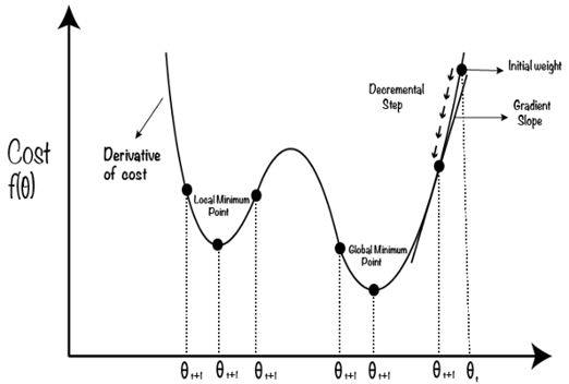
_{Source: An Efficient Optimization Technique for Training Deep Neural Networks.}

Generally, we are using an Optimizer to slightly change the weights and biases every time we make a backward step, and then measure the Cost in the next step with the next mini-batch of training observations.

If this x-axis represents our network’s parameters, we change them slightly every run in order to reach the global minimum, not just a local one, which is sub-optimal.

Our optimizer has various hyperparameters to help it bounce around in a healthier way, trying to avoid local minima as much as possible. We will discuss this soon.

Accuracy

Accuracy is another measure of a machine learning model’s efficacy. Depending on the task at hand, it is calculated as the percent of correct predictions out of total predictions made.

Both loss and accuracy serve as a measure for how well a model was able to learn. Intuitively, the accuracy quickly tells us how good our model is in what it was trained to do. It is important to remember that we train on minimizing validation loss, while we use accuracy as a secondary indicator for actual real-life success.

Basically, in a classification task, the accuracy is the amount of times the model classified correctly out of total attempts. In a regression task, it is the amount of projections that are close enough to the true Target, since we are dealing with continuous numbers. This “approved distance” between the projection and true Target to be considered “correct” is set by dividing the standard deviation of the true Target values in a batch with a given number we set in advance. A projected Target that falls within this boundary will be considered correct.

Accuracy works best when it is true to assume a normal distribution of the Target within the population. When the distribution is biased, such when our Target only manifests in a small part of the population (such as a rare illness) or when high accuracy is very important (such as the case when we cannot tolerate a “false positive”, i.e. we would not like to provide an expensive treatment to a healthy person)- in these cases a simple accuracy will tell us nothing. It will even provide us a false sense of security in our model, showing a high accuracy while in reality this is not the case. This is called the “accuracy paradox”^◆, and we can handle with it by using tools like the Confusion Matrix, showing Precision, Recall, F1 and ROC and lift curves, which all come to make the task of measuring the efficacy of classifying tasks more efficient. See a very good explanation of the subject here.

The Confusion Matrix is a table used to evaluate the performance of a classification model. It provides a clear summary of the model’s predictions and the actual outcomes based on a test dataset. A confusion matrix allows us to understand the model’s strengths and weaknesses in predicting different classes, as it indicates the amount of true positives and negative, and false positives and negatives in predicting a class.

The following table is taken from Wikipedia, and shows the Confusion Matrix itself (the first 9 cells at the top-left corner) and the various ratios one can calculate to better score his model’s efficacy in classifying observations:

_{Source: Wikipedia.}

Generally, we will prefer to use a model that shows the highest test accuracy measurements.

Backpropagation and Optimization

After performing a forward step as part of the training, we get outputs from the model’s output layer and compute our loss. Our goal is to minimize this number by tweaking the Network’s parameters to the optimal setting.

The process during which the Network’s parameters get tweaked is called backpropagation, and it is done by using an optimizer algorithm. It is performed iteratively, so we begin by moving forward into the Network layer by layer with input data. We then measure our training loss, and then start going back by tweaking our output layer’s weights and biases, go back to the previous layer, tweak its parameters and so forth until we tweak the first hidden layer’s parameters. We then perform another forward step using another batch of training observations. Step by step, the optimization algorithm finds the value of the parameters (weights and biases) that minimize the error when mapping inputs to outputs. 

Backpropagation was first introduced in 1970s and was popularized in 1989 by Rumelhart, Hinton and Williams in a paper called “Learning representations by back-propagating errors”^◆.

An important note: our goal in training is to reach the minimum value of the Cost Function. However, these functions are convex, meaning they have many local minima. The best training results are reached when we find the global minimum, and not just a local minimum. An optimizer’s job is to be able to bounce over such local minima the Network encounters during training and get to the global minimum, which represents the least amount of loss the Network can reach.

As mentioned above, the backpropagation process is performed by using an optimizer algorithm (or just “optimizer”). There are more than one kind of optimizer and they all affect the model’s ability to learn and the speed of training.

An optimizer is an algorithm that tweaks a Network’s parameters to minimize the loss. Each algorithm might be superior in different tasks and using a specific set of parameters (of the optimizer algorithm).

The main algorithms used in Neural Network parameter optimization are based on a family of optimization techniques called gradient descent.

A gradient is a commonly used term in optimization and machine learning^◆. It is a vector of partial derivatives of a function that has more than one input variable, and basically contains information of how a small change in each variable’s value influences the function’s result.

For the gradient descent parameter optimization process we calculate the partial derivative of each parameter (weight and bias) in each layer in relation to the Cost Function. The derivative of the Cost Function is its slope in a point and this tells us how each parameter needs to change in order to move in our desired direction. Since we would like to minimize the Cost Function, we will change a parameter slightly to decrease the function’s value.

The derivative is partial since we are able to make a separate calculation for each and every parameter relative to the Cost Function. We compute these values by using the chain rule of calculus^◆, that enables us to break the composite function that defines a Neural Network into its constituents, and further calculate the partial derivative of each parameter with regards to the Cost Function^◆. This creates a chain of gradients, connected by multiplication, to describe a parameter change’s influence on the Cost Function.

Basically, the chain rule means that we can break any nested parameter’s influence on the target function into one expression of multiplication that includes all the gradients from it to the Cost Function. In other words, a parameter’s change influences the Cost Function through its influence on all the parameters that stand between it and the Cost Function.

As mentioned above, after we know each parameter’s partial derivative, we can tweak it such that its new value will bring a smaller Cost Function (loss) result, which is our goal in training. This tweaking is done slightly differently, depending on the optimization technique we employ in our model.

Gradient descent refers to the basic situation when we send our entire input dataset into the Network. However, we usually prefer to send batches of observations, be it 64, 128 or 256 and not the entire dataset for better efficiency. When we send batches of samples into the Network, the tweaking process is called “stochastic gradient descent”^◆ (stochastic means “random”) and it is more efficient, since a smaller sample is enough to get an idea of each parameter’s gradient, we don’t need the whole sample^◆. In large datasets, this takes a fraction of the processing power to fulfill and we can use the other parts of the sample to enhance our learning.

The optimizers often make use of some hyperparameters of their own. We can further enhance an optimizer’s efficacy by adding a momentum algorithm, which remembers the previous parameter changes and performs the tweaking a bit more efficiently.

Another important optimizer hyperparameter is the learning rate. This parameter sets the size of the distance an optimized parameter’s value can move towards the minimum. A too high number and the value can swing to the other side and miss the minimum. A too low number and training will take much longer^◆.

Over the years, various enhancements were made to the gradient descent algorithm. The most well known examples are:

• Adagrad (Adaptive Gradient Descent) Deep Learning Optimizer- This algorithm tweaks the improves on the descent algorithm by not keeping the learning rate constant during training. Under Adagrad, the learning rate changes between epochs based on the model parameters’ change magnitude. The more the model’s parameters are changed, the smaller the learning rate gets.
  
• RMSprop (Root Mean Squared Propagation) Optimizer- the RMSprop optimizer is similar to the gradient descent algorithm but with momentum. It uses a decaying average of partial gradients in the adaptation of the step size for each parameter, which allows the algorithm to forget early gradients and focus on the most recently observed partial gradients seen during the progress of the search, overcoming the limitation of AdaGrad^◆.
  
• AdaDelta- this technique allows for per-dimension learning rate method for the stochastic gradient descent algorithm. Instead of accumulating all past squared gradients, Adadelta restricts the window of accumulated past gradients to a fixed size. This method saves us the need to set a learning rate as a hyperparameter prior to training^◆.
  
• Adam (Adaptive Moment Estimation)- this optimizer is a combination of the “Adagrad” and the “RMSprop” algorithms. Unlike maintaining a single learning rate through training using stochastic gradient descent, the Adam optimizer updates the learning rate for each network weight individually. This optimizer has several benefits, which explain why it is so widely used. It was adopted as a benchmark for deep learning papers and recommended as a default optimization algorithm. This algorithm is straightforward to implement, has faster running time, low memory requirements, and requires less tuning than any other optimization algorithm.^◆.

For a good and deeper explanation about optimizers, see here and here.

The following figure shows how different optimization algorithms performed on deep convolutional Neural Networks (CNNs), as done by the researches who proposed the Adam optimizer. The left figure shows loss reduction in the first three epochs, and the right shows the full picture over 45 epochs:

It is visible that in this test, Adam achieved a much lower loss than the other optimizers.

The following figure shows the general process of backpropagation:

A deep explanation of backpropagation is given here.

Problems with gradients

During backpropagation, we go back through a Neural Network’s hidden layers up to the first hidden one and multiply all the gradients in the way to achieve the desired influence on the Cost Function. The further back we go in deeper Networks, the longer the gradient chain gets and the smaller the gradient that influences the layers’ parameters becomes. This is because the gradients are multiplied with one another in expressions that grow as there are more layers in the way between a hidden layer and the output layer. This means that later layers’ parameters are updated with larger values than those of the first layers of which gradient gets smaller and smaller. It also means that if the gradients are too large or too small, something will go wrong as the multiplication magnifies their affect.

As the Network is built to be more complex (i.e. having more hidden layers), it becomes more important to avoid “exploding” and “vanishing” gradients, both resulting in a “dead network” that does not learn. Unbalanced gradients bring to one of these two negative outcomes:

• Exploding gradients- this problem occurs when the Neural Network’s gradients get too large. large gradient values can accumulate to the point where the Network’s parameters themselves get too large, causing gradient descents to oscillate without coming to the global minimum^◆.  This happens when the gradients get larger than 1 in a deep Network, and as the gradients get multiplied over the layers using the chain rule, they may become very large. Sometimes they get so big that they overflow the device’s memory, return NaN values and stop the learning process.
  
• Vanishing gradients- this problem occurs when the Network’s gradients get too small and approach zero, which eventually leaves some weights nearly unchanged, mainly in the first hidden layers. As a result, the gradient descent may never converge to the optimum and learning may not happen^◆. This can occur when our activation function’s output range is small, such as the Sigmoid that returns values in the range of [0, 1] in an ever-decreasing pace. In such cases, large inputs to this activation function will only cause a small change in its output, making the Sigmoid’s derivative very small as the input gets larger (in absolute terms). The following figure shows the Sigmoid (blue line) and its derivative (green line). We can see that as the larger (in absolute terms) the input value to the function gets, the smaller the derivative becomes:

We can tackle these problems in the following ways:

• Weight initialization- as explained above in “Weight Initialization Techniques”. We should match the weight initialization technique to the activation functions used in our Network.
  
• Gradient clipping- we set a positive and negative limit to the gradients’ size. If a gradient passes the limit, its value will be adjusted to the limit it crossed.
  
• Replacing the activation function- altering the Network’s architecture can assist with gradient problems. If we discovered that an activation function achieves sub-optimal results, we can change it and train using another one.

Regularization

Regularization describes the actions we can take in order to control our model’s complexity by influencing a Feature’s importance and/or the number of Features it uses.  The goal is to prevent overfitting and increase a model’s ability to generalize.

The basic rule is that simple models are generally preferable over complex ones. We seek to achieve a balance between fitting to (training on) the training sample and being able to generalize and predict (or in other words, the balance between overfitting and underfitting, finding the sweet spot in the bias-variance tradeoff). Large parameter values tend to bring to a high model variance, as defined in the “Bias-Variance Tradeoff” part above, and hamper learning. This is where regularization comes in.

A machine learning model’s regularization techniques reduce overfitting in two ways, which can either be used separately or together. The first is called Feature shrinkage and the other dimension (Feature) reduction. They both let the model train on all the input Features while slowly reducing the importance of what seems to be unimportant Features (i.e. unrelated to the Target) by diminishing the parameters that relate to such Features. The two methods mainly defer by the following traits:

• Feature shrinkage- this method is able to shrink a Features’s parameters all the way to zero, effectively removing Features from the final equation. This is a form of Feature selection.
  
• Dimension (feature) reduction- this method can decrease a model’s Feature parameter values but does not bring them to zero completely.

There are several ways to implement regularization in a machine learning model, which we will now discuss. The first two influence the Cost Function directly (L1-norm and L2-norm), while Dropout influences it indirectly. Early stopping to the training process once a condition is met, can also be applied and is considered a type of regularization since it stops the model once it starts overfitting (i.e. showing a low training loss and a higher test loss. In other words, when the model trains and reaches the point where it stops generalizing and starts to to learn the statistical noise in the training dataset^◆).

L1, L2 Regularization

Here, regularization happens as each method calculates an extra loss penalty on the model and adds it to its Cost Function we are trying to minimize. This extra cost is calculated on each Feature parameter such that large values (in absolute terms) are punished more by adding a larger “loss” to the Cost Function, pushing the Network to tweak them more during backpropagation, further reducing weights and biases (in absolute terms) as necessary.

Using an optimizer, we set a regularization strength parameter, lambda (?), in advance. This parameter is usually very small, 10^-5 to 10^-9 (depending on the task) and is used to scale the penalty, the regularization loss, we add to the Cost Function. We need to be careful when choosing lambda to avoid regularization that is too strong, causing our model to miss important Features. This, since the larger the lambda is, the larger the regularization penalty and the smaller the Feature parameters get.

The two regularization methods used are:

• L1-regularization (using “L1-norm”), a.k.a Least Absolute Shrinkage and Selection Operator (Lasso Regression) in regression problems- this Feature shrinkage technique reduces overfitting by shrinking the model’s parameters all the way to zero, completely disregarding some Features. It completely eliminates unimportant Features by subtracting a small amount from the parameter at each iteration. It calculates a “Manhattan Distance” by summing the parameters’ absolute values. Essentially, the L1-regularization penalizes the absolute value of our model’s weights and biases. Mathematically, it looks like this:

Where the w and b are each layer’s weights and biases.

• L2-regularization (using “L2-norm”), Ridge Regression in regression problems- this Feature reduction technique reduces overfitting by decreasing our model parameters’ sizes but never completely removes them (never reaches a weight or bias of zero). This means that less significant Features will still have some impact on the Target, albeit a very small one. L2-regularization calculates a “Euclidian Distance” by summing the square value of each parameter. This method helps in cases when our samples have Features that are highly correlated to each other (called “multicollinearity”), however it is not robust to outliers (due to the squaring, which will significantly influence the Cost Function). Mathematically, it looks like this:

Unlike L2-regularization, L1-regularization does not deal well with highly correlated Features. In such cases, it would select only one of the correlated Features arbitrarily, resulting in missing information. Unlike the L2, L1-regularization is robust to outliers.

We can get the best of both worlds by combining the two into one regularization technique, called “Elastic Net”, which is simply the addition of the two methods. Basically:

The following figure is important for understanding the difference between L1 and L2-regularization. It shows why the L1-regularization is able to completely remove Features (a Feature’s parameter is depicted by a ?) while L2-regularization only shrinks their parameters. Note that the turquoise shapes for this two-dimensional (two parameters) representation are created by each method’s equation under a constraint s (this represents our will to reach a balance between overfitting and underfitting using regularization), with lasso (left) built with absolute factor value and ridge regression (right) by squaring each Feature parameter (also as seen above):

In the following figure, the axes represent a two-dimensional plain of two Feature parameters, each represented by a beta (we assume 2 model factors for simplicity). It includes the following parts:

• Mean Squared Error ellipses- this is the model’s loss under various parameter values. Its elliptical shape is due to how it’s made, the means of summed squared errors for various values of ?1 and ?2. Every point on a red ellipse indicates the same loss value. The smaller the ellipse, the smaller the model’s loss. ?_hat is these ellipses’ center.
  
• Constraint regions- The turquoise shapes depict the the L1 and L2-regularization’s restrictions, as defined by a given constraint s. A model’s minimum loss, given such constraint, is found where a constraint region is tangent to an MSE ellipse.

Since the L1-regularization’s constraint boundaries (left chart) appear as vertices on the parameters’ axes, the meeting point of the loss and constraint regions can bring a weight to zero when they meet, resulting in ?₂ completely removed from the model’s equation in order to reach minimum loss. L2-regularization (right chart) does not show this quality due to its nature, and therefore only reduces a parameter’s value close to zero.

While it may seem that the process described above prefers a higher loss (a larger ellipse) when including regularization in the model, we actually reach a more “real” loss, since when applying regularization we help avoid overfitting (a seemingly low loss while training but a high loss when testing) and increase the model’s ability to generalize.

For a deeper explanation of regularization see here and here, and definitely see this.

As we can see, regularization gives us the freedom to start training a model with all the Features we think are related to the Target, and let it methodically diminish the relative importance of unimportant Features, bringing more weight to the truly important ones and keeping our model simpler.

Dropout

Dropout is another type of regularization, as it helps avoiding overfitting in our Network. A dropout layer basically acts as an interim layer between two layers, taking in the output of the layer neurons’ activation functions and randomly assigns zeros to some of them. This output, effectively with some disabled neuron outputs, is fed into the next layer as input.

The rationale behind Dropout is that it helps with Feature selection and increased ability to learn the true relationships in the population. This works by letting the Network train with missing inputs by totally erasing some parameters, forcing it to train with the ones left and achieve a projected Target. This causes the Network to spread the weights over more parameters and not to focus on the few ones it thinks are the most influential on the Target. This process should help with the Network’s ability to learn and generalize^◆.

We can also choose to only employ Dropout on the first few layers of a deep learning model. We should use whatever technique which best helps the Network’s ability to generalize.

We can see the general idea of Dropout in this figure:

_{Source: Analytics Vidhya.}

Generally, different regularization types should not be used together in the same model since they can interfere with each other.

Early stopping

Early stopping refers to the cessation of the training process once a condition is met. The goal of this procedure is to stop the model from fitting the training set too strongly and also to save wasted time on training an overfitting model which may have already passed its “sweet spot” of optimal training.

It is the simplest regularization method to understand, but finding the right rules is tricky and depends on the dataset and task, and also involves some trial and error.

There are at least several rules for early stopping we can use, which can be implemented concurrently. In the following examples, the first three are dynamic and the last two are static and set in advance:

• Stop when the validation performance indicators, loss or accuracy, have deteriorated or haven’t changed significantly for several epochs.
• Stop when validation performance indicators have risen above training performance indicators.
• Stop when the Network’s gradients “explode” or “vanish”.
• Setting maximum epochs for training as a hyperparameter.
• IBM also suggests possibly stopping training after a certain time has passed^◆.

Pseudorandomness

Machine learning models use a random distribution of numbers to manipulate input values and “learn” the true relationships between Features and a Target in the population. Randomness is used for shuffling the training, validation and test datasets in order to nullify any influence made by the observations’ order of appearance, when the task requires. Specifically in Neural Networks, randomness is used for weight initialization, k-fold cross validation, Dropout and in choosing a random batch of observations for feeding through the Network, which sits at the base of the Stochastic (random) Gradient Descent process.

In our model training process, we need to have a “random” pool of numbers that the model can draw from and use, but we need the pool to be constant and keep the same numbers in the same order every time we run the model, in order to have reproducibility. This is called “Pseudorandomness” and it is the result of performing the same algorithm on the same seed number, resulting in the same number pool every time.

We need to be able to reach the exact same result when running the same model more than once on the same inputs.

Therefore, a very important yet simple step in training a machine learning model is setting the program’s random seed to a fixed number. In Python, this is done by inserting the following row at the beginning of the script:

numpy.random.seed(a)

numpy.random.seed(a)

With “numpy” representing the Numpy package and “a” representing a seed number. If we don’t feed the method a number, it will use the system’s time at the moment of program run, which will result in our model having no reproducibility.

Conclusion

In this text we went over the main subjects relating to Neural Networks from top to bottom, starting with the theory, main obstacles, data preparation, NNs and their architecture, the “learning” process, performance measurement, model selection, regularization and more.

With a clearer understanding of machine learning and neural networks, it’s evident that this is a highly intricate yet promising field that offers us powerful tools for uncovering the hidden connections within vast datasets. By analyzing patterns and relationships in data, we can deepen our understanding of the world around us, make more informed predictions, and generate insights that were previously beyond our reach.

The potential of neural networks ignites the imagination, opening up seemingly infinite possibilities for innovation. Recent advances such as simultaneous translation, word-to-image generation, and even word-to-video applications demonstrate the astonishing capabilities of these models. While some researchers have made bold claims about the development of models that exhibit elements of consciousness^◆, we must remember that current machine learning models excel primarily at interpolation, meaning they are good at generalizing within known parameters.

However, the ability to extrapolate, to apply learned concepts to entirely new dimensions, remains a significant challenge for these systems^◆. The idea of machines taking over the world remains far-fetched, but there is no doubt that machine learning and neural networks offer immense value in the meantime. As we continue to refine these models, we can expect them to play an increasingly vital role in solving complex problems and driving technological progress across industries.

* * *